Download
1 / 32
320 likes | 436 Vues
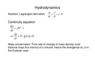
Hydrodynamics in High-Density Scenarios. Assumes local thermal equilibrium (zero mean-free-path limit) and solves equations of motion for fluid elements (not particles) Equations given by continuity, conservation laws, and Equation of State (EOS)

E N D
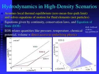
Hydrodynamics in High-Density Scenarios • Assumes local thermal equilibrium (zero mean-free-path limit) and solves equations of motion for fluid elements (not particles) • Equations given by continuity, conservation laws, and Equation of State (EOS) • EOS relates quantities like pressure, temperature, chemical potential, volume = direct access to underlying physics Kolb, Sollfrank & Heinz, hep-ph/0006129
Hydromodels can describe mT (pT) spectra • Good agreement with hydrodynamic prediction at RHIC & SPS (2d only) • RHIC: Tth~ 100 MeV, bT ~ 0.55 c
Tdec = 100 MeV Kolb and Rapp,PRC 67 (2003) 044903. Blastwave vs. Hydrodynamics Mike Lisa (QM04): Use it don’t abuse it ! Only use a static freeze-out parametrization when the dynamic model doesn’t work !!
Basics of hydrodynamics Hydrodynamic Equations Energy-momentum conservation Charge conservations (baryon, strangeness, etc…) For perfect fluids (neglecting viscosity), Need equation of state (EoS) P(e,nB) to close the system of eqs. Hydro can be connected directly with lattice QCD Energy density Pressure 4-velocity Within ideal hydrodynamics, pressure gradient dP/dx is the driving force of collective flow. Collective flow is believed to reflect information about EoS! Phenomenon which connects 1st principle with experiment
Tchemical Tchemical Input for Hydrodynamic Simulations Final stage: Hadronic interactions (cascade ?) Need decoupling prescription Intermediate stage: Hydrodynamics can be applied if thermalization is achieved. Need EoS (Lattice QCD ?) • Initial stage: • Pre-equilibrium, • Color Glass Condensate ? • Instead parametrization (a) for hydro simulations
Caveats of the different stages • Initial stage • Recently a lot of interest (Hirano et al., Heinz et al.) • Presently parametrized through initial thermalization time t0, initial entropy density s0 and a parameter (pre-equilibrium ‘partonic wind’) • QGP stage • Which EoS ? Maxwell construct with hadronic stage ? • Nobody uses Lattice QCD EoS. Why not ? • Hadronic stage • Do we treat it as a separate entity with its own EoS • Hadronic cascade allows to describe data without an a
Interface 1: Initial Condition • Need initial conditions (energy density, flow velocity,…) Initial time t0 ~ thermalization time • Take initial distribution • from other calculations • Parametrize initial • hydrodynamic field y y Hirano .(’02) x x x Energy density from NeXus. (Left) Average over 30 events (Right) Event-by-event basis e or s proportional to rpart, rcoll or arpart + brcoll
Main Ingredient: Equation of State One can test many kinds of EoS in hydrodynamics. EoS with chemical freezeout Typical EoS in hydro model H: resonance gas(RG) Q: QGP+RG p=e/3 Kolb and Heinz (’03) Hirano and Tsuda(’02) Latent heat PCE:partial chemical equiliblium CFO:chemical freeze out CE: chemical equilibrium
Interface 2: Hadronization Kolb, Sollfrank, Huovinen & Heinz; Hirano;… Hirano & Tsuda; Teaney; Kolb & Rapp Teaney, Lauret & Shuryak; Bass & Dumitru Ideal hydrodynamics QGP phase Tc Chemical Equilibrium EOS Partial Chemical Equilibrium EOS Tch Hadronic Cascade Hadron phase Tth Tth t
The Three Pillars of Experimental Tests to Hydrodynamics • Identified Spectra • Radial Flow in partonic and hadronic phase • Identified Elliptic Flow (v2) • Spatial to Momentum anisotropy, mostly in partonic phase • HBT results • Kinetic Freezeout Surface • Lifetime of Source • Conclusions from hydro • Early local thermalization • Viscosity, mean free path • Coupling, Collectivity
π-, K-, p : reasonable agreement • Best agreement for : Tdec= 100 MeVα = 0.02 fm-1 • α≠ 0 : importance of inital conditions • Only at low pT (pT < 1.5 – 2 GeV/c) • Failing at higher pT (> 2 GeV/c) expected: • Less rescattering Central Data Tdec = 165 MeV Tdec = 100 MeV Thermalization validity limit P.F. Kolb and R. Rapp, Phys. Rev. C 67 (2003) 044903 α : initial (at τ0) transverse velocity : vT(r)=tanh(αr)
π-, K-, p : apparent disagreement? STAR preliminary data • Predictions normalized to data • Limited range of agreement • Hydro starts failing at 62 GeV? • different feed-down treatment in data and hydro? • Different initial / final conditions than at 200 GeV ? • Lower Tdec at 62 GeV ? • Larger τ0 at 62 GeV ? • Increasing τ0 gives much better agreement! • Tdec = 100 MeV
Conclusions from spectra • Central spectra well described either by including a pre-equilibrium transverse flow or by using a hadron cascade for the hadronic phase. • Multistrange Baryons can be described with common decoupling temperature. Different result than blast wave fit. Blast wave fit is always better. • Centrality dependence poorly described by hydro • Energy dependence (62 to 200 GeV) indicates lower decoupling temperature and longer initial thermalization time at lower energy. System thermalizes slower and stays together longer.
z y x Collective anisotropic flow
Elliptic Flow(in the transverse plane)for a mid-peripheral collision Flow Y Out-of-plane In-plane Reaction plane Flow X Dashed lines: hard sphere radii of nuclei Re-interactions FLOW Re-interactions among what? Hadrons, partons or both? In other words, what equation of state?
Anisotropic Flow y f x z x Transverse plane Reaction plane A.Poskanzer & S.Voloshin (’98) “Flow” is not a good terminology especially in high pT regions due to jet quenching. 0th: azimuthally averaged dist. radial flow 1st harmonics: directed flow 2nd harmonics: elliptic flow …
Large spatial anisotropy turns intomomentum anisotropy, IF the particles interact collectively ! High pT protons Low pT protons
How does the system respond to the initial spatial anisotropy ? Free streaming Hydrodynamic expansion Ollitrault (’92) y f x INPUT Initial spatial anisotropy 2v2 Rescattering dN/df dN/df OUTPUT Final momentum anisotropy 0 f 2p 0 f 2p
Hydrodynamics describes the data Strong collective flow: elliptic and radial expansion with mass ordering Hydrodynamics: strong coupling, small mean free path, lots of interactions NOT plasma-like
# III: The medium consists of constituent quarks ? baryons mesons
v2 pT (GeV/c) How strong is the coupling ? Navier-Stokes type calculation of viscosity – near perfect liquid Viscous force ~ 0 Simple pQCD processes do not generate sufficient interaction strength (2 to 2 process = 3 mb)
Viscosity Primer • Remove your organic prejudices • Don’t equate viscous with “sticky” ! • Think instead of a not-quite-ideal fluid: • “not-quite-ideal” “supports a shear stress” • Viscosity hthen defined as • Dimensional estimate: • Viscosityincreases withtemperature • Large cross sections small viscosity
Ideal Hydrodynamics • Why the interest in viscosity? A.) Its vanishing is associated with the applicability of ideal hydrodynamics (Landau, 1955): B.) Successes of ideal hydrodynamics applied to RHIC data suggest that the fluid is “as perfect as it can be”, that is, it approaches the (conjectured) quantum mechanical limit See “A Viscosity Bound Conjecture”, P. Kovtun, D.T. Son, A.O. Starinets, hep-th/0405231
Consequences of a perfect liquid • All “realistic” hydrodynamic calculations for RHIC fluids to date have assumed zero viscosity h = 0 “perfect fluid” • But there is a (conjectured) quantum limit • Where do “ordinary” fluids sit wrt this limit? • RHIC “fluid” mightbe at ~2-3 on this scale (!) 400 times less viscous than water, 10 times less viscous than superfluid helium ! Motivated by calculation of lower viscosity bound in black hole via supersymmetric N=4 Yang Mills theory in AdS (Anti deSitter) space (conformal field theory) T=1012 K
plasma liquid ? gas liquid Viscosity in Collisions Hirano & Gyulassy, Teaney, Moore, Yaffe, Gavin, etc. supersymmetric Yang-Mills: s pQCD and hadron gas: s~ 1 d.o.f. in perfect liquid ? Bound states ?, constituent quarks ?, heavy resonances ?
Suggested Reading • November, 2005 issue of Scientific American “The Illusion of Gravity” by J. Maldacena • A test of this prediction comes from the Relativistic Heavy Ion Collider (RHIC) at BrookhavenNational Laboratory, which has been colliding gold nuclei at very high energies. A preliminary analysis of these experiments indicates the collisions are creating a fluid with very low viscosity. Even though Son and his co-workers studied a simplified version of chromodynamics, they seem to have come up with a property that is shared by the real world. Does this mean that RHIC is creating small five-dimensional black holes? It is really too early to tell, both experimentally and theoretically. (Even if so, there is nothing to fear from these tiny black holes-they evaporate almost as fast as they are formed, and they "live" in five dimensions, not in our own four-dimensional world.)
χ2 minimum result D->e 2σ 1σ 4σ Even charm flows • strong elliptic flow of electrons from D meson decays → v2D > 0 • v2c of charm quarks? • recombination Ansatz: (Lin & Molnar, PRC 68 (2003) 044901) • universal v2(pT) for all quarks • simultaneous fit to p, K, e v2(pT) a = 1 b = 0.96 c2/ndf: 22/27 • within recombination model: charm flows like light quarks!
Constraining medium viscosity h/s • Simultaneous description of STAR R(AA) and PHENIX v2 for charm. (Rapp & Van Hees, PRC 71, 2005) • Ads/CFT == h/s ~ 1/4p ~ 0.08 • Perturbative calculation of D (2pt) ~6 (Teaney & Moore, PRC 71, 2005) == h/s~1 • transport models require • small heavy quark relaxation time • small diffusion coefficient DHQ x (2pT) ~ 4-6 • this value constrains the ratio viscosity/entropy • h/s ~ (1.3 – 2) / 4p • within a factor 2 of conjectured lower quantum bound • consistent with light hadron v2 analysis • electron RAA ~ p0 RAA at high pT - is bottom suppressed as well?
An alternate idea (Abdel-Aziz & Gavin) Level of viscosity will affect the diffusion of momentum correlations kinematic viscosity QGP + mixed phase + hadrons T() Broadening from viscosity s = width of momentum covariance C in rapidity Abdel-Aziz & S.G effect on momentum diffusion: limiting cases: viscous liquid pQGP ~HRG~ 1 fm nearly perfect sQGP ~ (4 Tc)-1 ~ 0.1 fm wanted: rapidity dependence of momentum correlation function
STAR measurement we want: STAR measures: density correlation function may differ from rg maybe n 2* STAR, PRC 66, 044904 (2006) uncertainty range * 2* 0.08 s 0.3