Queuing Models
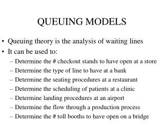
Queuing Models. Basic Concepts. QUEUING MODELS. Queuing is the analysis of waiting lines It can be used to: Determine the # checkout stands to have open at a store Determine the type of line to have at a bank Determine the seating procedures at a restaurant

Queuing Models
E N D
Presentation Transcript
Queuing Models Basic Concepts
QUEUING MODELS • Queuing is the analysis of waiting lines • It can be used to: • Determine the # checkout stands to have open at a store • Determine the type of line to have at a bank • Determine the seating procedures at a restaurant • Determine the scheduling of patients at a clinic • Determine landing procedures at an airport • Determine the flow through a production process • Determine the # toll booths to have open on a bridge
COMPONENTS OF QUEUING MODELS • Arrival Process • Waiting in Line • Service/Departure Process • Queue -- The waiting line itself • System -- All customers in the queuing area • Those in the queue • Those being served
The Queuing Process 1. Customers arrive according to some arrival pattern The Queue The System 2. Customers may have to wait in a queue 3. Customers are served according to some service distribution and depart 4 customers in the queue 7 customers in the system
ARRIVAL PROCESS • Deterministic or Probabilistic (how?) • Determined by # customers in system/balking? • Single or batch arrivals? • Priority or homogeneous customers? • Finite or infinite calling population?
THE WAITING LINE • One long line or several smaller lines • Jockeying allowed? • Finite or infinite line length? • Customers leave line before service? • Single or tandem queues?
THE SERVICE PROCESS • Single or multiple servers? • All servers serve at same rate? • Deterministic of probabilistic (how?) • Speed of service depends on line length? • FIFO/LIFO or some other service priority?
OBJECTIVE • To design systems that optimize some criteria • Maximizing total profit • Minimizing average wait time for customers • Meeting a desired service level
TYPICAL SERVICE MEASURES • L = Average Number of customers in the system • LQ = Average Number of customers in the queue • W = Average customer time in the system • WQ = Average customer waiting time in the queue • Pn = Probability n customers are in the system • = Average number of busy servers (utilization rate)
POISSON ARRIVAL PROCESS • REQUIRED CONDITIONS • Orderliness • at most one customer will arrive in any small time interval of t • Stationarity • for time intervals of equal length, the probability of n arrivals in the interval is constant • Independence • the time to the next arrival is independent of when the last arrival occurred
NUMBER OF ARRIVALS IN TIME t • Assume = the average number of arrivals per hour (THE ARRIVAL RATE) • For a Poisson process, the probability of k arrivals in t hours has the following Poisson distribution:
Time Between Arrivals • The average time between arrivals is 1/ • For a Poisson process, the time between arrivals in hours has the following exponential distribution: f(x) = e-t This means: P(next arrival occurs > t hours from now) = e-t P(next arrival occurs within t hours) = 1- e-t
POISSON SERVICE PROCESS • REQUIRED CONDITIONS • Orderliness • at most one customer will depart in any small time interval of t • Stationarity • for time intervals of equal length, the probability of completing n potential services in the interval is constant • Independence • the time to the completion of a service is independent of when it started • IS THIS A GOOD ASSUMPTION?
NUMBER OF POTENTIAL SERVICES IN TIME t • Unlike the arrival process, there must be customers in the system to have services • Assume = the average number of potential services per hour (SERVICE RATE) • For a Poisson process, the probability of k potential services in t hours has the following Poisson distribution:
THE SERVICE TIME • The average service time is 1/ • For a Poisson process, the service time has the following exponential distribution: f(x) = e-t This means: P(the service will take t more hours) = e-t P(service will be completed in t hours) = 1- e-t
TRANSIENT vs. STEADY STATE • Steady state is the condition that exists after the system has been operational for a while and wild fluctuations have been “smoothed out” • Until steady state occurs the system is in a transient state -- transiting to steady state • It is the long run steady state behavior that we will measure
CONDITIONS FOR STEADY STATE • For any queuing system to be stable the overall arrival rate must be less than the overall potential service rate, i.e. • For one server: < • For k servers with the same service rate: < k • For k servers with different service rates: < 1 + 2 + 3 + …+ k
STEADY STATEPERFORMANCE MEASURES • We’ve mentioned these before: • L = Average Number of customers in the system • LQ = Average Number of customers in the queue • W = Average customer time in the system • WQ = Average customer waiting time in the queue • Pn = Probability n customers are in the system • = Average number of busy servers
Little’s Laws • Little’s Laws relate L to W and LQ to WQ by: LITTLE’S LAWS L = λW LQ = λWQ
Relationship Between the System and the Queue (# in Sys) = (# in queue) + (# being served) • Thus, taking expected values of both sides: E(# in Sys) = E(# in queue) + E(# being served) L = Lq + • It can be shown that: ρ = λ/μ
Relationship Between the System and Queue Wait Times (Time in Sys) = (Time in queue) + (Service Time) • Thus, taking expected values of both sides: E(Time in Sys) = E(Time in queue) + E(Service Time) W = WQ + 1/μ • Thus, from last two slides and Little’s Laws, knowing one of L, W, Lq and Wq allows us to find the other values. Suppose we know L. LQ = L – λ/μ W = L/λ WQ = LQ/λ
CLASSIFICATION OF QUEUING SYSTEMS • Queuing systems are typically classified using a three symbol designation: (Arrival Dist.)/(Service Dist.)/(# servers) • Designations for Arrival/Service distributions include: • M = Markovian (Poisson process) • D = Deterministic (Constant) • G = General Sometimes the designation is extended to a 4th or 5th symbol to indicate Max queue length and # in population
Review • Components of a queuing system • Arrivals, Queue, Services • Assumptions for Poisson (Markovian) distribution • Requirements for Steady State • Overall service rate > Overall arrival rate • Steady State Performance Measures • L, Lq, W, Wq, pn’s, • Little’s Laws: L = λW and LQ = λWQ • System/Queue: L = LQ + λ/μ and W = WQ +1/μ • 3-5 component queue classification