Queuing Models in Economic Analyses
Understand queuing models in economic analyses with examples on determining servers, comparing situations, and deciding the optimal system based on cost and service criteria.

Queuing Models in Economic Analyses
E N D
Presentation Transcript
Queuing Models Economic Analyses
ECONOMIC ANALYSES • Each problem is different • Examples • To determine the minimum number of servers to meet some service criterion (e.g. an average of < 4 minutes in the queue) -- trial and error with M/M/k systems • To compare 2 or more situations -- • Consider the total (hourly) cost for each system and choose the minimum
Example 1Determining Optimal Number of Servers • Customers arrive according to a Poisson process to an electronics store at random at an average rate of 100 per hour. • Service times are exponential and average 5 min. • How many servers should be hired so that the average time of a customer waits for service is less than 30 seconds? • 30 seconds = .5 minutes = .00833 hours
Average service time1/ = 5 min. = 5/60 hr. = 60/5 =12/hr. ……….. How many servers? Arrival rate = 100/hr. GOAL: Average time in the queue, WQ < .00833hrs.
Input values for and First time WQ < .008333 12 servers needed .003999 Go to the MMkWorksheet
Example 2Determining Which Server to Hire • Customers arrive according to a Poisson process to a store at night at an average rate of 8 per hour. • The company places a value of $4 per hour per customer in the store. • Service times are exponential and the average service time that depends on the server. Server Salary Average Service Time • Ann $ 6/hr. 6 min. • Bill $ 10/hr. 5 min. • Charlie $ 14/hr. 4 min. • Which server should be hired?
Ann1/ = 6 min. A = 60/6 = 10/hr. LAnn = ? = 8/hr ANN Hourly Cost = $6 + 4LAnn
LAnn = 4 Ann1/ = 6 min. A = 60/6 = 10/hr. LAnn Hourly Cost = $6 + 4LAnn = 8/hr Hourly Cost = $6 + $4(4) = $22
Bill1/ = 5 min. A = 60/5 = 12/hr. LBill = ? = 8/hr BILL Hourly Cost = $10 + 4LBill
LBill = 2 Bill1/ = 5 min. B = 60/5 = 12/hr. LBill Hourly Cost = $10 + 4LBill = 8/hr LBill Hourly Cost = $10 + $4(2) = $18
Charlie1/ = 4 min. A = 60/5 = 15/hr. LCharlie = ? = 8/hr CHARLIE Hourly Cost = $14 + 4LCharlie
LCharlie = 1.14 Charlie1/ = 4 min. C = 60/4 = 15/hr. LCharlie Hourly Cost = $14 + 4LCharlie = 8/hr LCharlie 1.14 Hourly Cost = $14 + $4(1.14) = $18.56
Optimal HireBill • Ann --- Total Hourly Cost = $22 • Bill --- Total Hourly Cost = $18 • Charlie --- Total Hourly Cost = $18.56
Example 3What Kind of Line to Have • A fast food restaurant will be opening a drive-up window food service operation whose service distribution is exponential. • Customers arrive according to a Poisson process at an average rate of 24/hr. Three systems are being considered. • Customer waiting time is valued at $25/hr. • Each clerk makes $6.50/hr. • Each drive-thru lane costs $20/hr. to operate Which of the following systems should be used?
System 1 -- 1 clerk, 1 lane 1/ = 2 min. = 60/2 = 30/hr. Store = 24/hr. Total Hourly Cost Salary + Lanes + Wait Cost $6.50 + $20 + $25LQ
System 1 -- 1 clerk, 1 lane 1/ = 2 min. = 60/2 = 30/hr. LQ = 3.2 Store = 24/hr. Total Hourly Cost Salary + Lanes + Wait Cost $6.50 + $20 + $25(3.2) = $106.50 Total Hourly Cost Salary + Lanes + Wait Cost $6.50 + $20 + $25LQ
System 2 -- 2 clerks, 1 lane 1 Service System 1/ = 1.25 min. = 60/1.25 = 48/hr. Store = 24/hr. Total Hourly Cost Salary + Lanes + Wait Cost 2($6.50) + $20 + $25LQ
System 2 -- 2 clerks, 1 lane 1 Service System 1/ = 1.25 min. = 60/1.25 = 48/hr. LQ = .5 Store = 24/hr. Total Hourly Cost Salary + Lanes + Wait Cost 2($6.50) + $20 + $25(.5) = $45.50 Total Hourly Cost Salary + Lanes + Wait Cost 2($6.50) + $20 + $25LQ
System 3 -- 2 clerks, 2 lanes 1/ = 2 min. = 60/2 = 30/hr. Store Store = 24/hr. Total Hourly Cost Salary + Lanes + Wait Cost 2($6.50) + $40 + $25LQ
System 3 -- 2 clerks, 2 lanes 1/ = 2 min. = 60/2 = 30/hr. LQ = .152 Store Store = 24/hr. Total Hourly Cost Salary + Lanes + Wait Cost 2($6.50) + $40 + $25LQ Total Hourly Cost Salary + Lanes + Wait Cost 2($6.50) + $40 + $25(.152) = $56.80
Optimal • System 1 --- Total Hourly Cost = $106.50 • System 2 --- Total Hourly Cost = $ 45.50 • System 3 --- Total Hourly Cost = $ 58.80 Best option -- System 2
Example 4Which Store to Lease • Customers are expected to arrive by a Poisson process to a store location at an average rate of 30/hr. • The store will be open 10 hours per day. • The average sale grosses $25. • Clerks are paid $20/hr. including all benefits. • The cost of having a customer in the store is estimated to be $8 per customer per hour. • Clerk Service Rate = 10 customers/hr. (Exponential) Should they lease a Large Store ($1000/day, 6 clerks, no line limit) or a Small Store ($200/day, 2 clerks – maximum of 3 in store)?
Large Store 6Servers Unlimited QueueLength … = 30/hr. Lease Cost = $1000/day= $1000/10 = $100/hr. All customersget served!
Small Store 2Servers Maximum QueueLength = 1 Will join system if0,1,2 in the system Will not join thequeue if there are 3 customers in the system = 30/hr. Lease Cost = $200/day= $200/10 = $20/hr.
Hourly Profit Analysis Large Small Arrival Rate = 30 e = 30(1-p3) Hourly Revenue $25(Arrival Rate) (25)(30)=$750 $25e Hourly Costs Lease$100 $20 Server$20(#Servers) $120 $40 Waiting$8(Avg. in Store) $8L $8L Net Hourly Profit??
Large Store -- M/M/6 L 3.099143
Small Store -- M/M/2/3 p3 L e = (1-.44262)(30) = 16.7213
Hourly Profit Analysis Large Small Arrival Rate = 30 e = 16.7213 Hourly Revenue $25(Arrival Rate) $750 $25e=$418 Hourly Costs Lease$100 $20 Server$20(#Servers) $120 $40 Waiting$8(Avg. in Store) $25 $17 Net Hourly Profit$505 $341 Lease the Large Store
Example 5Which Machine is Preferable • Jobs arrive according to a Poisson process to an assembly plant at an average of 5/hr. • Service times do not follow an exponential distribution. • Two machines are being considered • (1) Mean service time of 6 min. ( = 60/6 = 10/hr.) standard deviation of 3 min. ( = 3/60 = .05 hr.) • (2) Mean service time of 6.25 min.( = 60/6.25 = 9.6/hr.); std. dev. of .6 min. ( = .6/60 = .01 hr.) Which of the two M/G/1designs is preferable?
Machine Comparisons Machine1 Machine 2 Prob (No Wait) -- P0 .5000.4792 Average Service Time6 min.6.25 min. Average # in System.8125.8065 Average # in Queue .3125.2857 Average Time in System.1625 hr..1613 hr. 9.75 min.9.68 min. Average Time in Queue.0625 hr..0571 hr. 3.75 min.3.43 min. Machine 2 looks preferable
Review • List Components of System • Develop a model • Use templates to get parameter estimates • Select “optimal” design