Process Capability
Process Capability. Process Capability. Process Capability is an important concept in SPC. Process capability examines -- the variability in process characteristics -- whether the process is capable of producing products which conforms to specifications. Process Capability.

Process Capability
E N D
Presentation Transcript
Process Capability • Process Capability is an important concept in SPC. Process capability examines -- the variability in process characteristics -- whether the process is capable of producing products which conforms to specifications
Process Capability • Process capability studies distinguish between conformance to control limits and conformance to specification limits (also called tolerance limits) -- if the process is in control, then virtually all points will remain within control limits -- staying within control limits does not necessarily mean that specification limits are satisfied -- specification limits are usually dictated by customers
Process Capability: Concepts • The following distributions show different process scenarios. Note the relative positions of the control limits and specification limits.
Process Capability: Concepts • In control and product meets specifications.Control limits are within specification limits UCL: Upper Control Limits LCL: Lower Control Limits USL: Upper Specification Limits LSL: Lower Specification Limits
Process Capability: Concepts • In control but some products do not meet specifications.Specification limits are within control limits
Data from process with mediumcapability relative capability Data from process with low capability Data from process with highcapability
Process capability: capability index • The capability index is defined as: Cp = (allowable range)/6 =T (Tolerance)/ 6= (USL - LSL)/6s The distribution of process quality is often assumed to be approximated with a normal distribution. P(x∈μ±3σ)=99.73%,
f (x) =0.5 =1 =2 x 0 f (x) x 1 2 0 Normal Distribution The normal distribution N(,2) has several distinct properties: --The normal distribution is bell-shaped and is symmetric --The mean, , is located at the centre -- is the standard deviation of the data The smaller ,the steeper the curve For same ,changing the value of μ is to move the curve without any change in its shape
0.9974 μ-3 μ+3 3 Principle The probability for X to fall within (-3,+3)is 99.74%, and the probability for falling outside this interval is only 0.26% which is considered almost impossible. That characteristic of normal distribution is called “3 principle”. Applying this principle in QM can judge whether there is abnormity appearing in the process, since three standard deviations above and below the process mean represent almost all the fluctuation range of the process. • X∼N(,2) • P{-<X<+}=(1)-(-1)=2(1)-1=0.6826 • P{-2<X<+2}=2(2)-1=0.9544 • P{-3<X<+3}=2(3)-1=0.9974
Process capability: capability index • The capability index (T/6) show how well a process is able to meet specifications. The higher the value of the index, the more capable is the process: -- Cp < 1 (process is unsatisfactory) -- 1 < Cp < 1.6 ( process is of medium relative capability) -- Cp > 1.6 (process shows high relative capability): better to analyze the actual specifications (Tolerance) and process technics to save resources in enhancing the process capability, such as the increased accuracy of equipment.
Process capability: process performance index • The capability index -- considers only the spread of the characteristic in relation to specification limits -- assumes two-sided specification limits • The product can be bad if the mean is not set appropriately. The process performance index takes account of the mean () and is defined as: Cpk = min[ (USL - )/3, ( - LSL)/3]
Process capability: process performance index • The process performance index can also accommodate one sided specification limits -- for upper specification limit: Cpk = (USL - )/3 -- for lower specification limit: Cpk = ( - LSL)/ 3
Process capability: the message • The message from process capability studies is: -- first reduce the variation in the process -- then shift the mean of the process towards the target This procedure is illustrated in the diagram below:
Basic Forms of Statistical Sampling for Quality Control • Sampling to determine if the process is within acceptable limits (Statistical Process Control). • Sampling to accept or reject the immediate lot of product at hand (Acceptance Sampling).
Process Control • Process Control is concerned with monitoring quality while the production or service is being conducted.
UCL Statistical Process Control -- Control Charts Normal Behavior LCL 1 2 3 4 5 6 Samples over time UCL Possible problem, investigate LCL 1 2 3 4 5 6 Samples over time UCL Possible problem, investigate LCL 1 2 3 4 5 6 Samples over time
Control charts • Processes that are not in a state of statistical control -- show excessive variations -- exhibit variations that change with time • A process in a state of statistical control is said to be statistically stable. Control charts are used to detect whether a process is statistically stable. Control charts differentiates between variations -- that is normally expected of the process due chance or common causes -- that change over time due to assignable or special causes
Control charts: common cause variations • Variations due to common causes -- have small effect on the process -- are inherent in the process because of: • the nature of the system • the way the system is managed • the way the process is organized and operated -- can only be removed by • making modifications to the process • changing the process -- are the responsibility of higher management
Control charts: special cause variations • Variations due to special causes are -- localized in nature -- exceptions to the system -- considered abnormalities -- often specific to a • certain operator • certain machine • certain batch of material, etc. • Investigation and removal of variations due to special causes are key to process improvement • Note:Sometimes the delineation between common and special causes may not be very clear.
Control charts: how they work • The principles behind the application of control charts are very simple and are based on the combined use of -- run charts -- hypothesis testing • The control limits most commonly used in organizations are plus and minus three standard deviations. We know from statistics that the chance that a sample mean will exceed three standad deviations, in either direction, due simply to chance variation, is less than 0.3 percent (i.e., 3 times per 1000 samples). Thus, the chance that a sample will fall above the UCL, or below the LCL because of natural random causes is so small that this occurrence is strong evidence of assignable variation.
Control charts: how they work • The procedure is to -- sample the process at regular intervals -- plot the statistic (or some measure of performance), e.g. • mean • range • variable • number of defects, etc. -- check (graphically) if the process is under statistical control -- if the process is not under statistical control, do something about it
Control charts: types of charts • Different charts are used depending on the nature of the charted data. Commonly used charts are: -- for continuous (variables) data • Shewhart sample mean ( -chart) • Shewhart sample range (R-chart) • Shewhart sample (X-chart) • Cumulative sum (CUSUM) • Exponentially Weighted Moving Average (EWMA) chart • Moving-average and range charts -- for discrete (attributes and countable) data • sample proportion defective (p-chart) • sample number of defectives (np-chart) • sample number of defects (c-chart) • sample number of defects per unit (u-chart)
Control charts: assumptions • Control charts make assumptions about the plotted statistic, namely -- it is independent, i.e. a value is not influenced by its past value and will not affect future values -- it is normally distributed, i.e. the data has a normal probability density function
Normal Probability Density Function The assumptions of normality and independence enable predictions to be made about the data.
Control charts: interpretation • Control charts are normal distributions with an added time dimension.
Control charts: interpretation • Control charts are run charts with superimposed normal distributions.
Control charts: run rules • Run rules are rules that are used to indicate out-of-statistical control situations. Typical run rules for Shewhart X-charts with control and warning limits are: -- a point lying beyond the control limits -- 2 consecutive points lying beyond the warning limits, namely within the area of 2 ~3 or even beyond the control limits -- 7 or more consecutive points lying on one side of the mean -- 5 or 6 or more consecutive points going in the same direction (indicates a trend) -- Other run rules can be formulated using similar principles
UCL CL LCL UCL CL LCL attention investigate Prompt action Trend
Control charts: run rules • If only chance variation is present in the process, the points plotted on a control chart will not typically exhibit any pattern. • If the points exhibit some systematic pattern, this is an indication that assignable variation may be present and corrective action should be taken.
Given: Compute control limits: Attribute Measurements (p-Chart)
Sample n Defectives p 1 100 4 0.04 2 100 2 0.02 3 100 5 0.05 4 100 3 0.03 5 100 6 0.06 6 100 4 0.04 7 100 3 0.03 8 100 7 0.07 9 100 1 0.01 10 100 2 0.02 11 100 3 0.03 12 100 2 0.02 13 100 2 0.02 14 100 8 0.08 15 100 3 0.03 Example of Constructing a p-chart: 1. Calculate the sample proportions, p (these are what can be plotted on the p-chart) for each sample.
Example of Constructing a p-chart: 2. Calculate the average of the sample proportions. 3. Calculate the standard deviation of the sample proportion
Example of Constructing a p-chart: 4. Calculate the control limits. UCL = 0.0924 LCL = -0.0204(or 0)
p 0.16 0.14 0.12 UCL 0.1 UCL 0.08 0.06 0.04 CL 0.02 0 Sample number 1 2 3 4 5 6 7 8 9 10 11 12 13 14 15 Example of Constructing a p-chart: 5. Plot the individual sample proportions and the control limits