Stereo vision and two-view geometry
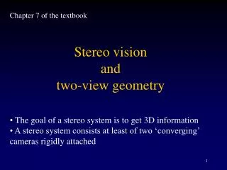
Chapter 7 of the textbook. Stereo vision and two-view geometry. The goal of a stereo system is to get 3D information A stereo system consists at least of two ‘converging’ cameras rigidly attached. One real example:. Three topics:. stereo geometry: epipolar geometry

Stereo vision and two-view geometry
E N D
Presentation Transcript
Chapter 7 of the textbook Stereo vision and two-view geometry • The goal of a stereo system is to get 3D information • A stereo system consists at least of two ‘converging’ cameras rigidly attached
One real example: Three topics: • stereo geometry: epipolar geometry • geometric relation between two images • correspondence • pixels (pts) in different images from the same pt • reconstruction (triangulation) • 3d coordinate of the pt
Intuitive epipolar geomegtry Entirely characterized by the so-called epipolar geometry • Geometric concepts: • epipole: the image of the other camera center • epipolar plane: plane defined by the two camera centers and the space pt • epipolar lines: intersection of the epipolar plane and image plane • pencil of epipolar lines and planes • baseline: distance between two camera centers
u u’ O O epipolar plane epipolar line epipole
Algebraic characterisation of the epipolar geometry: the fundamental matrix Given a correspondence pair u and u’, where F is 3 by 3 • Proof sketch: follow the geometric construction. • compute the epipole in the second image • compute the pt at infinity (or ray direction), reproject it onto the second • define the epipolar line by these two pts • use anti-symmetric matrix for cross-product • Assume the camera projection matrices are P=(I 0) and P’=(A a), • it can be shown that F = [a] A. • The procedure is the same even if P is of general form.
Properties of the fundamental matrix F: • rank of F • ker(F) • how many d.o.f. • l’=F u • l = …
Stereo Vision by ‘traditional’ calibrated approach two (or more) cameras rigidly attached = stereo rig = stereo system Traditional (calibrated) stereo approach: • calibration of each camera w.r.t. the same object: P and P’ • (optional) rectification • disparity map using F • 3D reconstruction Correspondence using F (computed from P and P’)
Correspondence (discussed later) • 3D reconstruction : trianglulation Same equation as the calibration, but unknowns are now xi, yi, zi instead of cij
Triangulation: u u’ O O’
‘Modern’ uncalibrated approach:Epipolar geometry by point correspondences – two-view geometry Because of NB: it is more powerful, ‘calibration’ needs 3d info, point-correspondence does not, but not 3d reconstruction
Given compute F • 8 pts algorithm • 7 pts algorithm (minimal data) • (optimal and robust sol.)
8-point algorithm (unstable) expand rewrite for N points rewrite
linear sol by svd with ||f||=1: f=v9 • F’, rank enforcement afterwards by svd!
7-point algorithm • one parameter solution by svd • from the vanishing determinant, get a cubic equation
Warning: unnormalised 8 pt algorithm is unstable!!! Normalisation 8 pt algorithm To make the average point as close as possible to (1,1,1)! • normalisation by transformations • linear solution for • rank enforcement • denormalisation
Data normalisation: each image data is normlised independently!
Summary (or a unified view) of all methods of computation of the fundamental matrix
The epipolar geometry gives only a constraint, but not yet a unique solution to the question: where is the corresponding point in the second image of a given point in the first image? • disparity: difference in image position of the same space pt • disparity map: dense pixel-to-pixel corrrespondences • stereo rectification: make the epipolar lines horizontal • an option to speed up the computation of disparity map
Rectification of a stereo pair of images: two images are transformed (by a projective transformation in image plane or by a camera rotation around the center).
New rectified image plane • equivalent to a plane parallel to the base line • T and T’ can be computed from F, but many possibilities • only an option, simplify the computation!
Matching by correlation: or Very often ZNCC (Zero Normalized Cross Correlation), on normalised images instead of I and I’, Convert all (2n+1)(2n+1) elements from a matrix into a vector of dim (2n+1)(2n+1)
Two points u and u’ are in correspondence if • ZNCC(u,u’) is big enoug (close to 1) • dist(u’, Fu) is small enough (a few pixels)
Correspondence by correlation: • For each point u, compute all correlations in a neighborhood u+d with a window size s • Take the pixel having the highest correlation score as the correspondence • Cross-validate the correspondence in the opposite direction from the second to the first image neighborhood Correlation window Cross-validate
When applied to ‘interest points’, sparse correspondence When applied to every pixel, dense disparity map
Using more cameras to remove match ambiguity: a system of 3 cameras 1 3 2
What can we do more with F? • Without calibration, what can we get? • When calibrated, essential matrix, its decomposition
From uncalibrated F Calibrated E
Essential matrix: fundamental matrix for the calibrated points Relationship between E and F E = [t] R From F = [a] A Decomposition of the essential matrix into R and t The extra algebraic constraint: the equal singular values (more complicated) for E
Decomposition of E Two factorisation Twisted pair Two translation
Summary of modern two-view approach: • Given internal calibration K and K’ (more advanced studies allow us to remove this step by self-calibration that we will not handle) • Compute F from point correspondences • Compute E • Decompose E to obtain R and t • Obtain P and P’ • Triangulation
x u u’ O Never forget the coplanar case! O When space points are planar, a homography relating u and u’ It is therefore a ‘collineation’ for COPLANAR points!
From P=(I 0) , P’=(A a) and a known plane p^Tx=0, to get H So that Or, the homography can be computed from at least 4 corresponding Points, do it! The homography uniquely determines point correspondences Unlike the fundamental matrix! But only for coplanar points.
This homography leads to one important application: Panoramic image or image mosaicing • the 3D scene is planar • the camera is rotating around the center (similar to rectification) Example at HK airport (virtual tour), QuicktimeVR Realviz, stitcher, step-by-step http://iris.usc.edu/home/iris/elkang/iris-04/reports/2/techreport2.html
The images are related by a homography if the 3d scene is planar:
x Rotating the camera around the center is equivalent to a homographical Transformation of the image plane: A pencil of lines cut by two lines A star of lines cut by two planes
Compositing algorithm or mosacing algorithm: • Compute point correspondences • Compute the projective transformation between the two views • Warp the first image onto the second • Color-blend the overlapping areas
Quick-time VR Outward-looking large-scale environnement Inward-looking small object Example of the virtual tour of HK airport: http://www.hkairport.com/eng/index.jsp
Automatic computation of the fundamental matrix Chicken-egg problem: we need corresponding points to compute F, we need F to establish correspondences … Simultaneous automatic computation of correspondences and F
Illustrative example of fitting a line to a set of 2D points • the least squares solution (orthogonal regression) is optimal when no outliers • but it is becoming very fragile to outliers
Robust line fitting Fit a line to 2D data containing ‘bad points’---outliers Solving two pbs: 1. A line fit to the data; 2. A classification of the data into ‘inliers’ and ‘outliers’ ‘inliers’: valid or good data satisfying the ‘line’ model ‘outliers’: bad data not satisfying the model
How to find the best line? repeating • randomly draw 2 data points • compute a line Li from these 2 points • compute the distance to the line Li for each data point • determine inliers/outliers by a threshold t • compute the number of inliers Si • select the Li having the largest Si • re-estimate the final line using all inliers then
Fischler and Bolles 1981 RANSAC (random sample consensus) repeating • randomly draw a sample of s data • initiate the model Mi • compute the distance to the model for each data pt • determine inliers/outliers by the threshold t • compute the size of inliers Si • select the Mi having the largest Si • re-estimate using all inliers then
The complete algorithm of automatic computation of F: • detect points of interest in each image • compute the correspondences using correlation based method • RANSAC using 7-pt algo. • (non-linear optimal estimation on the final inliers: • this is unnecessary in many cases, so just an option)
RANSAC using 7-pt algo to compute F repeating • randomly draw a sample of 7 corresponding points • compute Fi • compute the distance to Fi for each corresponding pt • determine inliers/outliers by the threshold t • compute the size of inliers Si • select the Fi having the largest Si • re-estimate the final F using all inliers then
How many times to repeat? p Probability of success (only inliers) Outlier proportion s Sample size Ex: 99.9% success rate, 50% outliers s=2, N=17 s=4, N=72 s=6, N=293 s=7, N=588 s=8, N=1177
Robust statistics From least-squares method to robust statistics (Ransac,least median of squares (LMS)) Handle ‘big errors’---outliers! This is useful not only for computing F, but also for automatically computing a mosaicing of images!