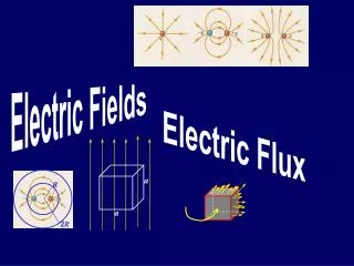
Electric Fields 4
Electric Fields 4. Overview. Session 4: covers electricity in water which includes electric field concepts/field form terms (e.g. voltage gradient, power density), field mapping, and electric field patterns as a function of electrode size and applied voltage. Session Purposes.

Electric Fields 4
E N D
Presentation Transcript
Overview • Session 4: covers electricity in water which includes electric field concepts/field form terms (e.g. voltage gradient, power density), field mapping, and electric field patterns as a function of electrode size and applied voltage.
Session Purposes • Familiarize participants with electric field terms, characteristics, and measurements. • Investigate factors the change the shape and intensity of electric fields.
Session Objectives • Define the “field form” terms voltage gradient, current density, and power density and relate them to a cube of water in an electric field (water conductivity covered previously) • Use the field form Ohm’s Law and power equations • Describe the electric field around electrodes of different sizes and shapes • Predict changes in an electric field with different electrode spacing • Describe equipment needed and procedure to map an electric field
Electric Field Measurements • The voltage difference along some length of an electric field (as a centimeter) can be measured with a voltage gradient probe and meter • Current density cannot be measured directly
Electric Field Measurements • Water conductivity can be measured
How Do We Measure Power Density? Power Density (D) = E x J But J cannot be measured! Second form Ohm’s Law: E = J/σ So, rearranging the equation: J = E x σ and thus, D = E x J = E x (E x σ) = E 2 x σ
Graphic Representation of the Power Density and 2nd Form Ohm’s Law Equations
Electric Field Mapping Set-up Reference electrode
Plot of Voltage Distribution S-shaped curve
Deriving Voltage Gradients = line tangent to curve indicating slope
Plot of Voltage Gradient Distribution U-shaped curve
Comprehensive Mapping of the Electric Field
Isopotential Surface Current pathway
More charge carriers per cm2, thus greater current density close to electrodes
A Field Map Defined by Voltage Gradients Lengthwise Distance from Boat Cathode (m) Crosswise distance from central axis of boat (m) From Miranda and Kratochvil (2008)
Voltage Gradient Meter and Probe • Meter:if a DC waveform is used, a typical commercial multimeter would read voltage gradient. If, however, the field is generated by pulsed DC or AC, then either an oscilloscope or a specialized multimeter capable of reading pulsed DC peak voltage or AC peak voltage is required.
Voltage Gradient Meter and Probe • Probe: These probes are commonly made of PVC containing two wires with fittings for attaching to the appropriate meter. Wire ends are bared and inserted through the bottom of the probe at a 1 cm pacing. The anode side of the probe is painted red. • See Voltage Gradient Probe construction.pdf
Mapping an Electric Field Map • Your task in mapping is to record voltage gradients by distance from the anode (center of electrode or from the electrode surface) • You may be interested in depth or horizontal extent • Typically a fully detailed map is not needed but rather a couple vectors from an anode, as lateral and forward
Mapping an Electric Field Map (continued) • When mapping, rotating the voltage gradient probe results in voltage gradient varying from zero to a maximum • zero corresponds to the equipotential surface, that is, the electrodes on the probe are aligned along a surface (as a bird on a wire) • the maximum voltage gradient reading occurs when the probe electrodes are aligned across (perpendicular to) the equipotential surface (similar to a bird spanning two power lines with its wings)
Mapping an Electric Field Map (continued) • Here are four short videos of field mapping- Measure Backpack Electric Field Measure Boat Electric Field 1 Measure Boat Electric Field 2 Measure Boat Electric Field 3
Mapping an Electric Field Map (continued) • How-to: see Making Electric Field Measurements.pdf
Field Map Attributes • Because voltage gradient and water conductivity can be measured, power density can be calculated at any point in the field (D = E 2 x σ) • An electric field defined by voltage gradients can therefore also be defined by power density
Field Map Attributes (continued) • Voltage gradient magnitudes are directly related to applied voltage • For example, an electric field has been mapped at an applied voltage to the electrodes of 200 V. By doubling the applied voltage from 200 to 400 V, all voltage gradient contours double (the 1 V/cm contour doubles to 2 V/cm, the 0.05 V/cm contour doubles to 0.1 V/cm, etc.) • Power density magnitudes also are related to applied voltage • Doubling applied voltage will quadruple (4x) power density because of the squared term in the equation: D = E 2 x σ • A field location having voltage gradient of 2 V/cm in a σ = 100 µS/cm has a D = 400 µW/cm3; doubling applied voltage changes the voltage gradient to 4 V/cm and increases D to 1,600 µW/cm3
Field Map Attributes (continued) • Voltage gradient patterns are a result of electrode geometry and arrangement • Voltage gradient magnitudes and patterns are not affected by changes in water conductivity versus One boom anode Two boom anodes
Field Map Attributes (continued) • Here is a vector of voltage gradients from the center of a Wisconsin ring anode, 216 V applied, distance from array center to waterline of bow (cathode) is 270 cm. The field intensity drops off exponentially and is described by the equation on the graph. One use for this graph is to determine how far from the anode center a threshold value occurs. If, for example, in a particular water conductivity, you need 0.72 V/cm for immobilization, that voltage gradient occurs about 87 cm lateral of the array center.
Field Map Attributes (continued) • The Excel tool “Electric Field Mapper” fits a predictive power regression equation to your electric field mapping data (voltage gradients at distances). You can explore the shape of electric fields across different electrode configurations or across a range of applied voltages. • This tool also allows you to merge the field map with lab information on thresholds for capture-prone responses. That merging results in an estimate of effective field size that can be used for standardization. More on this later.
Field Map Attributes (continued) • But what about power densities? Do power densities change with varying water conductivities? • Yes, proportionally; Power Density = E 2 x σ • If water conductivity doubles, power densities double • The reason for this is because current densities vary proportionally to σ
Field Mapping • An example of a field map data form is “Field Map form.pdf” • Additional discussion of methods and equipment in Kolz (1993) • The effective range rule-of-thumb holds that the edge of the effective field is approximately 0.1 V/cm
Field Mapping • Effective range can be increased, obviously, by applying more power to the electrodes (achieved through the voltage control on the control box • Due to the non-linear decrease in voltage gradient from the electrodes, doubling the applied voltage does not double the effective field size, increases in size often around 20% instead Profiles of voltage gradient (E) and the square of voltage gradient (E 2; essentially power density) for two spheres having diameters of 15.2 and 27.7 cm (Kolz 1993)
Field Mapping Explorations • There are two Excel tools that you can use to explore electric field map dynamics • Go to Electrofishing with Power v 2, the “Electric Fields” tab; you may investigate electric fields provided or enter the field you measured on your gear; the “Documentation” tab has an explanation and examples that can be followed • Go to Spherical Electrode Fields to investigate the question of which size diameter of spherical electrodes to use; follow the documentation first
Electric Field Pattern Experiments Using metal filings
NEG NEG
Cathode is directly wired; hull not directly wired
Cathode skirt (in connection with the hull); appearance as an isolation cathode
Common configuration for “streambank shockers” Earth as the cathode.
Next Step “Power Transfer Model and Standardization” (Session 5)