Chapter 2. Transmission Line Theory
2.05k likes | 6.07k Vues
Chapter 2. Transmission Line Theory. Sept. 29 th , 2008. 2.1 Transmission Lines. A transmission line is a distributed-parameter network, where voltages and currents can vary in magnitude and phase over the length of the line. Lumped Element Model for a Transmission Line

Chapter 2. Transmission Line Theory
E N D
Presentation Transcript
Chapter 2. Transmission Line Theory Sept. 29th, 2008
2.1 Transmission Lines • A transmission line is a distributed-parameter network, where voltages and currents can vary in magnitude and phase over the length of the line. Lumped Element Model for a Transmission Line • Transmission lines usually consist of 2 parallel conductors. • A short segment Δz of transmission line can be modeled as a lumped-element circuit.
Figure 2.1 Voltage and current definitions and equivalent circuit for an incremental length of transmission line. (a) Voltage and current definitions. (b) Lumped-element equivalent circuit.
R = series resistance per unit length for both conductors • L = series inductance per unit length for both conductors • G = shunt conductance per unit length • C = shunt capacitance per unit length • Applying KVL and KCL,
Dividing (2.1) by Δz and Δz 0, Time-domain form of the transmission line, or telegrapher, equation. • For the sinusoidal steady-state condition with cosine-based phasors,
Wave Propagation on a Transmission Line • By eliminating either I(z) or V(z): where the complex propagation constant. (α = attenuation constant, β = phase constant) • Traveling wave solutions to (2.4): Wave propagation in +z directon Wave propagation in -z directon
Applying (2.3a) to the voltage of (2.6), • If a characteristic impedance, Z0, is defined as • (2.6) can be rewritten
Converting the phasor voltage of (2.6) to the time domain: • The wavelength of the traveling waves: • The phase velocity of the wave is defined as the speed at which a constant phase point travels down the line,
Lossless Transmission Lines • R = G = 0 gives or • The general solutions for voltage and current on a lossless transmission line:
The wavelength on the line: • The phase velocity on the line:
2.2 Field Analysis of Transmission Lines • Transmission Line Parameters Figure 2.2 (p. 53)Field lines on an arbitrary TEM transmission line.
The time-average stored magnetic energy for 1 m section of line: • The circuit theory gives • Similarly,
Power loss per unit length due to the finite conductivity (from (1.130)) • Circuit theory (H || S) • Time-average power dissipated per unit length in a lossy dielectric (from (1.92))
Circuit theory • Ex 2.1 Transmission line parameters of a coaxial line • Table 2.1
The Telegrapher Equations Derived form Field Analysis of a Coaxial Line • Eq. (2.3) can also be obtained from ME. • A TEM wave on the coaxial line: Ez = Hz = 0. • Due to the azimuthal symmetry, no φ-variation ə/əφ = 0 • The fields inside the coaxial line will satisfy ME. where
Since the z-components must vanish, From the B.C., Eφ = 0 at ρ = a, b Eφ = 0 everywhere
The voltage between 2 conductors The total current on the inner conductor at ρ = a
Propagation Constant, Impedance, and Power Flow for the Lossless Coaxial Line • From Eq. (2.24) • For lossless media, • The wave impedance • The characteristic impedance of the coaxial line Ex 2.1
Power flow ( in the z direction) on the coaxial line may be computed from the Poynting vector as • The flow of power in a transmission line takes place entirely via the E & H fields between the 2 conductors; power is not transmitted through the conductors themselves.
2.3 The Terminated Lossless Transmission Lines The total voltage and current on the line
The total voltage and current at the load are related by the load impedance, so at z = 0 • The voltage reflection coefficient: • The total voltage and current on the line:
It is seen that the voltage and current on the line consist of a superposition of an incident and reflected wave. standing waves • WhenΓ= 0 matched. • For the time-average power flow along the line at the point z:
When the load is mismatched, not all of the available power from the generator is delivered to the load. This “loss” is return loss (RL): RL = -20 log|Γ| dB • If the load is matched to the line, Γ= 0 and |V(z)| = |V0+| (constant) “flat”. • When the load is mismatched,
A measure of the mismatch of a line, called the voltage standing wave ratio (VSWR) (1< VSWR<∞) • From (2.39), the distance between 2 successive voltage maxima (or minima) is l = 2π/2β = λ/2 (2βl = 2π), while the distance between a maximum and a minimum is l = π/2β = λ/4. • From (2.34) with z = -l,
At a distance l = -z, Transmission line impedance equation
Special Cases of Terminated Transmission Lines • Short-circuited line ZL = 0 Γ= -1
Figure 2.6 (a) Voltage, (b) current, and (c) impedance (Rin = 0 or ) variation along a short-circuited transmission line.
Open-circuited line ZL = ∞ Γ= 1
Figure 2.8 (a) Voltage, (b) current, and (c) impedance (Rin = 0 or ) variation along an open-circuited transmission line.
Terminated transmission lines with special lengths. • If l = λ/2, Zin = ZL. • If the line is a quarter-wavelength long, or, l = λ/4+ nλ/2 (n = 1,2,3…), Zin = Z02/ZL. quarter-wave transformer
Figure 2.9 (p. 63)Reflection and transmission at the junction of two transmission lines with different characteristic impedances.
2.4 The Smith Chart • A graphical aid that is very useful for solving transmission line problems. Derivation of the Smith Chart • Essentially a polar plot of the Γ(= |Γ|ejθ). • This can be used to convert from Γto normalized impedances (or admittances), and vice versa, using the impedance (or admittance) circles printed on the chart.
If a lossless line of Z0 is terminated with ZL, zL = ZL/Z0 (normalized load impedance), • Let Γ= Γr +jΓi, and zL = rL + jxL.
The Smith chart can also be used to graphically solve the transmission line impedance equation of (2.44). • If we have plotted |Γ|ejθ at the load, Zin seen looking into a length l of transmission line terminates with zLcan be found by rotating the point clockwise an amount of 2βl around the center of the chart.
Smith chart has scales around its periphery calibrated in electrical lengths, toward and away from the “generator”. • The scales over a range of 0 to 0.5 λ.
Ex 2.2 ZL = 40+j70,l = 0.3λ, find Γl, Γin and Zin Figure 2.11 (p. 67)Smith chart for Example 2.2.
The Combined Impedance-Admittance Smith Chart • Since a complete revolution around the Smith chart corresponds to a line length of λ/2, a λ/4 transformation is equivalent to rotating the chart by 180°. • Imaging a give impedance (or admittance) point across the center of the chart to obtain the corresponding admittance (or impedance) point.
Ex 2.3ZL = 100+j50, YL, Yin ? when l = 0.15λ Figure 2.12 (p. 69)ZY Smith chart with solution for Example 2.3.
The Slotted Line • A transmission line allowing the sampling of E field amplitude of a standing wave on a terminated line. • With this device the SWR and the distance of the first voltage minimum from the load can be measured, from this data ZL can be determined. • ZL is complex 2 distinct quantities must be measured. • Replaced by vector network analyzer.
Assume for a certain terminated line, we have measured the SWR on the line and lmin, the distance from the load to the first voltage minimum on the line. • Minimum occurs when • The phase of Γ = • Load impedance
Ex 2.4 • With a short circuit load, voltage minima at z = 0.2, 2.2, 4.2 cm • With unknown load, voltage minima at z = 0.72, 2.72, 4.72 cm • λ = 4 cm, • If the load is at 4.2 cm, lmin = 4.2 – 2.72 = 1.48 cm = 0.37 λ
Figure 2.14 (p. 71)Voltage standing wave patterns for Example 2.4. (a) Standing wave for short-circuit load. (b) Standing wave for unknown load.
2.5 The Quarterwave Transformer Impedance Viewpoint • For βl = (2π/λ)(λ/4) = π/2 • In order for Γ = 0, Zin = Z0
Ex 2.5 Frequency Response of a Quarter-Wave Transformer • RL = 100, Z0 = 50
Figure 2.17 (p. 74)Reflection coefficient versus normalized frequency for the quarter-wave transformer of Example 2.5.
The Multiple Reflection Viewpoint Figure 2.18 (p. 75)Multiple reflection analysis of the quarter-wave transformer.