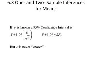
Inferences About Means
Inferences About Means. Chapter 23. Objectives. Construct confidence intervals for a population mean Conduct hypothesis tests for a population mean Examine the t-model used for inferences about means Use both critical t-value and P-values to make a decision about the null hypothesis.

Inferences About Means
E N D
Presentation Transcript
Inferences About Means Chapter 23
Objectives • Construct confidence intervals for a population mean • Conduct hypothesis tests for a population mean • Examine the t-model used for inferences about means • Use both critical t-value and P-values to make a decision about the null hypothesis. • Take a second look at the correct interpretation of a confidence interval.
Let’s Jump Into an Example A coffee machine dispenses coffee into paper cups. You’re supposed to get 10 ounces of coffee, but the amount varies slightly from cup to cup. Here are the amounts measured in a random sample of 20 cups. Is there evidence that the machine is shortchanging customers? n = 20, sample mean = 9.845, sample standard deviation = 0.199
Step 1: Hypothesis Claim to be tested – is the machine cheating customers (i.e. is the average amount of coffee dispensed by the machine less than 10 ounces)? Ho: m = 10.0 ounces Ha: m < 10.0 ounces • Notice that the hypothesis is about the population mean, m, not the sample mean, . • The null hypothesis again contains the condition of equality. • The alternative hypothesis may be one-sided ( < or >) or two-sided ( )
Step 2: Model We need to specify the model we will use to test the null hypothesis. We need to state our assumptions and check any corresponding conditions. Assumption #1: Data values are independent. Conditions to check: 1. Randomization Condition 2. 10% Condition Assumption # 2: Normal Population Assumption
Step 3: Mechanics Can we apply the normal model as we did with proportions? The Central Limit Theorem tells us that the sampling model for has a standard deviation of We do not have an estimate of the standard deviation of the population. What can we do to solve this problem?
Step 3: Mechanics (cont.) We could use the standard deviation of the sample deviation to estimate the standard deviation of the population. Thus, However, s is going to vary from sample to sample. This introduces variation in the denominator of our test statistic, which will have implications for our P-value and margin of error, especially for small samples. The shape of the model varies and is no longer normal. How can we account for this extra uncertainty?
Step 3: Mechanics (cont.) Solution – we can compensate for this added uncertainty (i.e. variability) by finding P-values and critical values using the t-distribution instead of the normal distribution as we did with proportions. Just as there is a z-score associated with the Normal distribution, there is a t-value associated with the t-distribution.
Important Properties of the Student’s t Distribution • The Student t distribution is different for different sample sizes. • The Student t distribution has the same general bell shape as the standard normal distribution; its wider shape reflects greater variability that is expected when s is used to estimate s. • The Student t distribution has a mean of t=0.
Important Properties of the Student’s t Distribution (cont.) • The standard deviation of the Student t distribution varies with the sample size and is greater than 1 (unlike the standard normal distribution, which has s =1). • As the sample size n gets larger, the Student t distribution gets closer to the standard normal distribution. • t-distributions are identified by their degrees of freedom, df= n -1.
Normal Population Assumption • Student’s t-model requires that the data are from a population that follows the normal model • Sufficient to check the Nearly Normal Condition – the data come from a distribution that is unimodal and symmetric. Make a histogram to check this condition. • Conclusion may depend on sample size • Small sample (n <15), if you find outliers or strong skewness, don’t use these methods • Moderate sample (n between 15 and 40), t-model will work well as long as distribution is unimodal and symmetric. • Large sample (n > 40), t-model can be used even if the data are skewed.
Our Example • Histogram of amounts dispensed per cup. • We hope to see a roughly mound-shaped, symmetric distribution without skewness or outliers.
One Sample t-test for the Mean The conditions have been met, therefore we can test the hypothesis Ho: m = 10.0 ounces using the statistic Our example:
Step 4: Conclusion The first part of the conclusion is to make a decision about the null hypothesis. Methods for making a decision about the null hypothesis. • Critical t-value method • P-value method
Critical t-value Method • Compare the t-statistic we have calculated to the critical t-value associated with a specific level of significance. • The critical value associated with a 5% significance level and df=19 is -1.729. (Be sure to look in the one tailed column for a one-sided alternative and the two tailed column for a two-sided alternative). Negative values are used when we are working on the left side of the distribution. • The area to the left (or right) of the critical value is called the critical region.
Critical t-value Method (cont.) • If the t-statistic falls in the critical region of the distribution reject the null. • If the t-statistic is not in the critical region Fail to Reject the null. • Our test statistic of -3.48 falls to the left of the critical value of -1.729, therefore we reject the null hypothesis.
P-value Method • Reject null if P-value < significance level a, fail to reject null if P-value > a. • T-Table includes only selected values of a. • Specific P-values usually cannot be found. • Use table to identify limits that contain the P-value. • Some calculators and computer programs will find exact P-values. • In our example we know that the P-value will be less than 0.005. We know that 0.005 is less than 0.05, therefore we reject the null hypothesis.
Final Conclusion Our test statistic of -3.48 falls in the critical region created by the critical value of -1.729, therefore we reject the null hypothesis. There is strong evidence that the mean amount of coffee dispensed by this machine is less than the stated 10 fluid ounces. What is the true population mean?
Confidence Interval for Population Mean When the conditions are met, we are ready to find the confidence interval for the population mean, m. The confidence interval is Where the standard error of the mean is, . The critical value depends on the particular confidence level, that you specify and on the number of degrees of freedom, n-1, which we get from the sample size.
Confidence Interval Example Let’s build a 95% confidence interval for the mean amount of coffee dispensed from the machine. The conditions are satisfied so we can use a t-model with (n-1) 19 degrees of freedom and find a one-sample t-interval for the mean. Calculating from the data: n = 20, = 9.845, s = 0.199 The standard error of is:
Confidence Interval Example (cont.) The 95% critical value is So the margin of error is Confidence interval is estimate +/_ margin of error or , recall that the sample mean is 9.845 so we have (9.75, 9.94). We are 95% confident that the machine dispenses an average of between 9.75 and 9.94 fluid ounces of coffee per cup.
Cautions About Interpreting Confidence Intervals • Don’t say, “95% of all cups of coffee contain between 9.75 and 9.94 ounces. • Don’t say, “We are 95% confident that a randomly selected cup of coffee will contain between 9.75 and 9.94 ounces. • Don’t say, “The average amount of coffee is 9.845 ounces 95% of the time. • Don’t say, “95% of all samples will have mean amounts of coffee between 9.75 and 9.94 ounces.
Example – Confidence Interval Hoping to lure more shoppers downtown, a city builds a new public parking garage in the central business district. The city plans to pay for the structure through parking fees. During a two-month period (44 weekdays), daily fees collected averaged $126, with a standard deviation of $15.
Example – Confidence Intervals (cont.) A.) What assumptions must you make in order to use these statistics for inference? B.) Write a 90% confidence interval for the mean daily income this parking garage will generate. C.) Explain in context what this confidence interval means. D.) Explain what “90% confidence” means in this context. E.) The consultant who advised the city on this project predicted that parking revenues would average $130 per day. Based on you confidence interval, do you think the consultant could have been correct? Why?
Example – Hypothesis Test #1 A company with a large fleet of cars hopes to keep gasoline costs down, and sets a goal of attaining a fleet average greater than 26 miles per gallon. To see if the goal is being met they check the gasoline usage for 50 company trips chosen at random, finding a mean of 26.50 mpg and a standard deviation of 4.83 mpg. Is this strong evidence that they have attained their fuel economy goal?
Example – Hypothesis Test #2 Forty subjects followed the Weight Watchers diet for a year. Their weight changes are summarized by these statistics: = -6.6lb, s = 10.8 lb. Use a 1% significance level to test the claim that the diet has no effect. Based on the results, does the diet appear to be effective?
Assignment • Wednesday’s lecture will include instruction on inferences about means in SPSS necessary for data analysis assignment #3, so COME TO CLASS!!! • Try the following problems from Ch. 23: • #3, 7, 9, 15, 17, 21, 23, 25, and 31
Remaining Assignments • Quiz # 6 – Monday, May 1st. Will cover chapters 21 and 23. • Data Assignment #3 Due on Wednesday, May 5th. • Exam #3 – Wednesday, May 5th. Will cover chapters 19, 20, 21 and 23.