Download

1 / 263
2.66k likes | 2.89k Vues
QSM 754 SIX SIGMA APPLICATIONS AGENDA. Day 1 Agenda. Welcome and Introductions Course Structure Meeting Guidelines/Course Agenda/Report Out Criteria Group Expectations Introduction to Six Sigma Applications Red Bead Experiment Introduction to Probability Distributions

E N D
Day 1 Agenda • Welcome and Introductions • Course Structure • Meeting Guidelines/Course Agenda/Report Out Criteria • Group Expectations • Introduction to Six Sigma Applications • Red Bead Experiment • Introduction to Probability Distributions • Common Probability Distributions and Their Uses • Correlation Analysis
Day 2 Agenda • Team Report Outs on Day 1 Material • Central Limit Theorem • Process Capability • Multi-Vari Analysis • Sample Size Considerations
Day 3 Agenda • Team Report Outs on Day 2 Material • Confidence Intervals • Control Charts • Hypothesis Testing • ANOVA (Analysis of Variation) • Contingency Tables
Day 4 Agenda • Team Report Outs on Practicum Application • Design of Experiments • Wrap Up - Positives and Deltas
Class Guidelines • Q&A as we go • Breaks Hourly • Homework Readings • As assigned in Syllabus • Grading • Class Preparation 30% • Team Classroom Exercises 30% • Team Presentations 40% • 10 Minute Daily Presentation (Day 2 and 3) on Application of previous days work • 20 minute final Practicum application (Last day) • Copy on Floppy as well as hard copy • Powerpoint preferred • Rotate Presenters • Q&A from the class
Learning Objectives • Have a broad understanding of statistical concepts and tools. • Understand how statistical concepts can be used to improve business processes. • Understand the relationship between the curriculum and the four step six sigma problem solving process (Measure, Analyze, Improve and Control).
Customer Critical To Quality (CTQ) Criteria • Breakthrough Improvements • Fact-driven, Measurement-based, Statistically Analyzed Prioritization • Controlling the Input & Process Variations Yields a Predictable Product • 6s = 3.4 Defects per Million Opportunities • Phased Project: Measure, Analyze, Improve, Control • Dedicated, Trained BlackBelts • Prioritized Projects • Teams - Process Participants & Owners What is Six Sigma? • A Philosophy • A Quality Level • A Structured Problem-Solving Approach • A Program
Sweet Fruit Design for Manufacturability ProcessEntitlement Bulk of Fruit Process Characterization and Optimization Low Hanging Fruit Seven Basic Tools Ground Fruit Logic and Intuition POSITIONING SIX SIGMA THE FRUIT OF SIX SIGMA
VALUE STREAM TO THE CUSTOMER WASTE DUE TO INCAPABLE PROCESSES • PROCESSES WHICH PROVIDE PRODUCT VALUE IN THE CUSTOMER’S EYES • FEATURES OR CHARACTERISTICS THE CUSTOMER WOULD PAY FOR…. • WASTE SCATTERED THROUGHOUT THE VALUE STREAM • EXCESS INVENTORY • REWORK • WAIT TIME • EXCESS HANDLING • EXCESS TRAVEL DISTANCES • TEST AND INSPECTION Waste is a significant cost driver and has a major impact on the bottom line... UNLOCKING THE HIDDEN FACTORY
Common Six Sigma Project Areas • Manufacturing Defect Reduction • Cycle Time Reduction • Cost Reduction • Inventory Reduction • Product Development and Introduction • Labor Reduction • Increased Utilization of Resources • Product Sales Improvement • Capacity Improvements • Delivery Improvements
All critical characteristics (Y) are driven by factors (x) which are “upstream” from the results…. Attempting to manage results (Y) only causes increased costs due to rework, test and inspection… Understanding and controlling the causative factors (x) is the real key to high quality at low cost... Y = f(x) The Focus of Six Sigma…..
INSPECTION EXERCISE The necessity of training farm hands for first class farms in the fatherly handling of farm livestock is foremost in the minds of farm owners. Since the forefathers of the farm owners trained the farm hands for first class farms in the fatherly handling of farm livestock, the farm owners feel they should carry on with the family tradition of training farm hands of first class farms in the fatherly handling of farm livestock because they believe it is the basis of good fundamental farm management. How many f’s can you identify in 1 minute of inspection….
INSPECTION EXERCISE The necessity of* training f*arm hands f*or f*irst class f*arms in the f*atherly handling of* f*arm livestock is f*oremost in the minds of* f*arm owners. Since the f*oref*athers of* the f*arm owners trained the f*arm hands f*or f*irst class f*arms in the f*atherly handling of* f*arm livestock, the f*arm owners f*eel they should carry on with the f*amily tradition of* training f*arm hands of* f*irst class f*arms in the f*atherly handling of* f*arm livestock because they believe it is the basis of* good f*undamental f*arm management. How many f’s can you identify in 1 minute of inspection….36 total are available.
Traditional Six Sigma “SIX SIGMA TAKES US FROM FIXING PRODUCTS SO THEY ARE EXCELLENT, TO FIXING PROCESSES SO THEY PRODUCE EXCELLENT PRODUCTS” Dr. George Sarney, President, Siebe Control Systems SIX SIGMA COMPARISON
Objective • Define the problem and verify the primary and secondary measurement systems. • Identify the few factors which are directly influencing the problem. • Determine values for the few contributing factors which resolve the problem. • Determine long term control measures which will ensure that the contributing factors remain controlled. Phase1: Measurement Characterization Phase 2: Analysis Breakthrough Strategy Phase 3: Improvement Optimization Phase4: Control IMPROVEMENT ROADMAP
Measurements are critical... • If we can’t accurately measure something, we really don’t know much about it. • If we don’t know much about it, we can’t control it. • If we can’t control it, we are at the mercy of chance.
WHY STATISTICS?THE ROLE OF STATISTICS IN SIX SIGMA.. • WE DON’T KNOW WHAT WE DON’T KNOW • IF WE DON’T HAVE DATA, WE DON’T KNOW • IF WE DON’T KNOW, WE CAN NOT ACT • IF WE CAN NOT ACT, THE RISK IS HIGH • IF WE DO KNOW AND ACT, THE RISK IS MANAGED • IF WE DO KNOW AND DO NOT ACT, WE DESERVE THE LOSS. DR. Mikel J. Harry • TO GET DATA WE MUST MEASURE • DATA MUST BE CONVERTED TO INFORMATION • INFORMATION IS DERIVED FROM DATA THROUGH STATISTICS
WHY STATISTICS?THE ROLE OF STATISTICS IN SIX SIGMA.. • Ignorance is not bliss, it is the food of failure and the breeding ground for loss. DR. Mikel J. Harry • Years ago a statistician might have claimed that statistics dealt with the processing of data…. • Today’s statistician will be more likely to say that statistics is concerned with decision making in the face of uncertainty. Bartlett
WHAT DOES IT MEAN? • Sales Receipts • On Time Delivery • Process Capacity • Order Fulfillment Time • Reduction of Waste • Product Development Time • Process Yields • Scrap Reduction • Inventory Reduction • Floor Space Utilization Random Chance or Certainty…. Which would you choose….?
Learning Objectives • Have a broad understanding of statistical concepts and tools. • Understand how statistical concepts can be used to improve business processes. • Understand the relationship between the curriculum and the four step six sigma problem solving process (Measure, Analyze, Improve and Control).
Learning Objectives • Have an understanding of the difference between random variation and a statistically significant event. • Understand the difference between attempting to manage an outcome (Y) as opposed to managing upstream effects (x’s). • Understand how the concept of statistical significance can be used to improve business processes.
WELCOME TO THE WHITE BEAD FACTORY • HIRING NEEDS • BEADS ARE OUR BUSINESS • PRODUCTION SUPERVISOR • 4 PRODUCTION WORKERS • 2 INSPECTORS • 1 INSPECTION SUPERVISOR • 1 TALLY KEEPER
STANDING ORDERS • Follow the process exactly. • Do not improvise or vary from the documented process. • Your performance will be based solely on your ability to produce white beads. • No questions will be allowed after the initial training period. • Your defect quota is no more than 5 off color beads allowed per paddle.
WHITE BEAD MANUFACTURING PROCESS PROCEDURES • The operator will take the bead paddle in the right hand. • Insert the bead paddle at a 45 degree angle into the bead bowl. • Agitate the bead paddle gently in the bead bowl until all spaces are filled. • Gently withdraw the bead paddle from the bowl at a 45 degree angle and allow the free beads to run off. • Without touching the beads, show the paddle to inspector #1 and wait until the off color beads are tallied. • Move to inspector #2 and wait until the off color beads are tallied. • Inspector #1 and #2 show their tallies to the inspection supervisor. If they agree, the inspection supervisor announces the count and the tally keeper will record the result. If they do not agree, the inspection supervisor will direct the inspectors to recount the paddle. • When the count is complete, the operator will return all the beads to the bowl and hand the paddle to the next operator.
INCENTIVE PROGRAM • Low bead counts will be rewarded with a bonus. • High bead counts will be punished with a reprimand. • Your performance will be based solely on your ability to produce white beads. • Your defect quota is no more than 7 off color beads allowed per paddle.
PLANT RESTRUCTURE • Defect counts remain too high for the plant to be profitable. • The two best performing production workers will be retained and the two worst performing production workers will be laid off. • Your performance will be based solely on your ability to produce white beads. • Your defect quota is no more than 10 off color beads allowed per paddle.
OBSERVATIONS……. WHAT OBSERVATIONS DID YOU MAKE ABOUT THIS PROCESS….?
The Focus of Six Sigma….. All critical characteristics (Y) are driven by factors (x) which are “downstream” from the results…. Attempting to manage results (Y) only causes increased costs due to rework, test and inspection… Understanding and controlling the causative factors (x) is the real key to high quality at low cost... Y = f(x)
Learning Objectives • Have an understanding of the difference between random variation and a statistically significant event. • Understand the difference between attempting to manage an outcome (Y) as opposed to managing upstream effects (x’s). • Understand how the concept of statistical significance can be used to improve business processes.
Learning Objectives • Have a broad understanding of what probability distributions are and why they are important. • Understand the role that probability distributions play in determining whether an event is a random occurrence or significantly different. • Understand the common measures used to characterize a population central tendency and dispersion. • Understand the concept of Shift & Drift. • Understand the concept of significance testing.
Why do we Care? • An understanding of Probability Distributions is necessary to: • Understand the concept and use of statistical tools. • Understand the significance of random variation in everyday measures. • Understand the impact of significance on the successful resolution of a project.
Phase1: Measurement Characterization Phase 2: Analysis Breakthrough Strategy Phase 3: Improvement Optimization Phase4: Control IMPROVEMENT ROADMAPUses of Probability Distributions Project Uses • Establish baseline data characteristics. • Identify and isolate sources of variation. • Demonstrate before and after results are not random chance. • Use the concept of shift & drift to establish project expectations.
Focus on understanding the concepts Visualize the concept Don’t get lost in the math…. KEYS TO SUCCESS
Measurements are critical... • If we can’t accurately measure something, we really don’t know much about it. • If we don’t know much about it, we can’t control it. • If we can’t control it, we are at the mercy of chance.
Types of Measures • Measures where the metric is composed of a classification in one of two (or more) categories is called Attribute data. This data is usually presented as a “count” or “percent”. • Good/Bad • Yes/No • Hit/Miss etc. • Measures where the metric consists of a number which indicates a precise value is called Variable data. • Time • Miles/Hr
COIN TOSS EXAMPLE • Take a coin from your pocket and toss it 200 times. • Keep track of the number of times the coin falls as “heads”. • When complete, the instructor will ask you for your “head” count.
R e s u l t s f r o m 1 0 , 0 0 0 p e o p l e d o i n g a c o i n t o s s 2 0 0 t i m e s . R e s u l t s f r o m 1 0 , 0 0 0 p e o p l e d o i n g a c o i n t o s s 2 0 0 t i m e s . C o u n t F r e q u e n c y C u m u l a t i v e C o u n t 6 0 0 1 0 0 0 0 y 5 0 0 c n e u y 4 0 0 q c e n r e F u 3 0 0 5 0 0 0 q e Cumulative Frequency v e i r t F a 2 0 0 l u m u 1 0 0 C 0 0 7 0 8 0 9 0 1 0 0 1 1 0 1 2 0 1 3 0 7 0 8 0 9 0 1 0 0 1 1 0 1 2 0 1 3 0 Cumulative Percent " H e a d C o u n t " R e s u l t s f r o m 1 0 , 0 0 0 p e o p l e d o i n g a c o i n t o s s 2 0 0 t i m e s . C u m u l a t i v e P e r c e n t Cumulative count is simply the total frequency count accumulated as you move from left to right until we account for the total population of 10,000 people. Since we know how many people were in this population (ie 10,000), we can divide each of the cumulative counts by 10,000 to give us a curve with the cumulative percent of population. 1 0 0 t n e c r e P e 5 0 v i t a l u m u C 0 7 0 8 0 9 0 1 0 0 1 1 0 1 2 0 1 3 0 " H e a d C o u n t " COIN TOSS EXAMPLE
R e s u l t s f r o m 1 0 , 0 0 0 p e o p l e d o i n g a c o i n t o s s 2 0 0 t i m e s C u m u l a t i v e P e r c e n t This means that we can now predict the change that certain values can occur based on these percentages. Note here that 50% of the values are less than our expected value of 100. This means that in a future experiment set up the same way, we would expect 50% of the values to be less than 100. 1 0 0 t n e c r e P e 5 0 v i t a l u m u C 0 7 0 8 0 9 0 1 0 0 1 1 0 1 2 0 1 3 0 COIN TOSS PROBABILITY EXAMPLE
R e s u l t s f r o m 1 0 , 0 0 0 p e o p l e d o i n g a c o i n t o s s 2 0 0 t i m e s . C o u n t F r e q u e n c y 6 0 0 5 0 0 y 4 0 0 c n e u 3 0 0 q e r F 2 0 0 1 0 0 0 7 0 8 0 9 0 1 0 0 1 1 0 1 2 0 1 3 0 " H e a d C o u n t " R e s u l t s f r o m 1 0 , 0 0 0 p e o p l e d o i n g a c o i n t o s s 2 0 0 t i m e s . C u m u l a t i v e P e r c e n t 1 0 0 t n e c r e P e 5 0 v i t a l u m u C 0 7 0 8 0 9 0 1 0 0 1 1 0 1 2 0 1 3 0 " H e a d C o u n t " COIN TOSS EXAMPLE We can now equate a probability to the occurrence of specific values or groups of values. For example, we can see that the occurrence of a “Head count” of less than 74 or greater than 124 out of 200 tosses is so rare that a single occurrence was not registered out of 10,000 tries. On the other hand, we can see that the chance of getting a count near (or at) 100 is much higher. With the data that we now have, we can actually predict each of these values.
PROCESS CENTERED ON EXPECTED VALUE 6 0 0 % of population = probability of occurrence SIGMA (s ) IS A MEASURE OF “SCATTER” FROM THE EXPECTED VALUE THAT CAN BE USED TO CALCULATE A PROBABILITY OF OCCURRENCE 5 0 0 If we know where we are in the population we can equate that to a probability value. This is the purpose of the sigma value (normal data). y 4 0 0 c n e u 3 0 0 q e r F 2 0 0 s 1 0 0 0 7 0 8 0 9 0 1 0 0 1 1 0 1 2 0 1 3 0 NUMBER OF HEADS 58 65 72 79 86 93 100 107 114 121 128 135 142 SIGMA VALUE (Z) -6 -5 -4 -3 -2 -1 0 1 2 3 4 5 6 CUM % OF POPULATION .003 .135 2.275 15.87 50.0 84.1 97.7 99.86 99.997 COIN TOSS PROBABILITY DISTRIBUTION
WHAT DOES IT MEAN? • Common Occurrence • Rare Event What are the chances that this “just happened” If they are small, chances are that an external influence is at work that can be used to our benefit….
Probability and Statistics • “the odds of Colorado University winning the national • title are 3 to 1” • “Drew Bledsoe’s pass completion percentage for the last • 6 games is .58% versus .78% for the first 5 games” • “The Senator will win the election with 54% of the popular • vote with a margin of +/- 3%” • Probability and Statistics influence our lives daily • Statistics is the universal lanuage for science • Statistics is the art of collecting, classifying, • presenting, interpreting and analyzing numerical • data, as well as making conclusions about the • system from which the data was obtained.
A sample is just a subset of all possible values sample population • Since the sample does not contain all the possible values, there is some uncertainty about the population. Hence any statistics, such as mean and standard deviation, are just estimates of the true population parameters. Population Vs. Sample (Certainty Vs. Uncertainty)
Inferential Statistics Descriptive Statistics Descriptive Statistics is the branch of statistics which most people are familiar. It characterizes and summarizes the most prominent features of a given set of data (means, medians, standard deviations, percentiles, graphs, tables and charts. Descriptive Statistics describe the elements of a population as a whole or to describe data that represent just a sample of elements from the entire population
Inferential Statistics Inferential Statistics is the branch of statistics that deals with drawing conclusions about a population based on information obtained from a sample drawn from that population. While descriptive statistics has been taught for centuries, inferential statistics is a relatively new phenomenon having its roots in the 20th century. We “infer” something about a population when only information from a sample is known. Probability is the link between Descriptive and Inferential Statistics
6 0 0 5 0 0 4 0 0 y c n e 3 0 0 u q e r F 2 0 0 s 1 0 0 0 7 0 8 0 9 0 1 0 0 1 1 0 1 2 0 1 3 0 58 65 72 79 86 93 100 107 114 121 128 135 142 -6 -5 -4 -3 -2 -1 0 1 2 3 4 5 6 .003 .135 2.275 15.87 50.0 84.1 97.7 99.86 99.997 WHAT DOES IT MEAN? WHAT IF WE MADE A CHANGE TO THE PROCESS? Chances are very good that the process distribution has changed. In fact, there is a probability greater than 99.999% that it has changed. And the first 50 trials showed “Head Counts” greater than 130? NUMBER OF HEADS SIGMA VALUE (Z) CUM % OF POPULATION