Fundamentals of Microelectronics
1.1k likes | 1.4k Vues
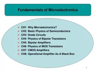
Fundamentals of Microelectronics. CH1 Why Microelectronics? CH2 Basic Physics of Semiconductors CH3 Diode Circuits CH4 Physics of Bipolar Transistors CH5 Bipolar Amplifiers CH6 Physics of MOS Transistors CH7 CMOS Amplifiers CH8 Operational Amplifier As A Black Box.

Fundamentals of Microelectronics
E N D
Presentation Transcript
Fundamentals of Microelectronics • CH1 Why Microelectronics? • CH2 Basic Physics of Semiconductors • CH3 Diode Circuits • CH4 Physics of Bipolar Transistors • CH5 Bipolar Amplifiers • CH6 Physics of MOS Transistors • CH7 CMOS Amplifiers • CH8 Operational Amplifier As A Black Box
Chapter 5 Bipolar Amplifiers • 5.1 General Considerations • 5.2 Operating Point Analysis and Design • 5.3 Bipolar Amplifier Topologies • 5.4 Summary and Additional Examples
Bipolar Amplifiers CH5 Bipolar Amplifiers
Voltage Amplifier • In an ideal voltage amplifier, the input impedance is infinite and the output impedance zero. • But in reality, input or output impedances depart from their ideal values. CH5 Bipolar Amplifiers
Input/Output Impedances • The figure above shows the techniques of measuring input and output impedances. CH5 Bipolar Amplifiers
Input Impedance Example I • When calculating input/output impedance, small-signal analysis is assumed. CH5 Bipolar Amplifiers
Impedance at a Node • When calculating I/O impedances at a port, we usually ground one terminal while applying the test source to the other terminal of interest. CH5 Bipolar Amplifiers
Impedance at Collector • With Early effect, the impedance seen at the collector is equal to the intrinsic output impedance of the transistor (if emitter is grounded). CH5 Bipolar Amplifiers
Impedance at Emitter • The impedance seen at the emitter of a transistor is approximately equal to one over its transconductance (if the base is grounded). CH5 Bipolar Amplifiers
Three Master Rules of Transistor Impedances • Rule # 1: looking into the base, the impedance is r ifemitter is (ac) grounded. • Rule # 2: looking into the collector, the impedance is ro if emitter is (ac) grounded. • Rule # 3: looking into the emitter, the impedance is 1/gm if base is (ac) grounded and Early effect is neglected. CH5 Bipolar Amplifiers
Biasing of BJT • Transistors and circuits must be biased because (1) transistors must operate in the active region, (2) their small-signal parameters depend on the bias conditions. CH5 Bipolar Amplifiers
DC Analysis vs. Small-Signal Analysis • First, DC analysis is performed to determine operating point and obtain small-signal parameters. • Second, sources are set to zero and small-signal model is used. CH5 Bipolar Amplifiers
Notation Simplification • Hereafter, the battery that supplies power to the circuit is replaced by a horizontal bar labeled Vcc, and input signal is simplified as one node called Vin. CH5 Bipolar Amplifiers
Example of Bad Biasing • The microphone is connected to the amplifier in an attempt to amplify the small output signal of the microphone. • Unfortunately, there’s no DC bias current running thru the transistor to set the transconductance. CH5 Bipolar Amplifiers
Another Example of Bad Biasing • The base of the amplifier is connected to Vcc, trying to establish a DC bias. • Unfortunately, the output signal produced by the microphone is shorted to the power supply. CH5 Bipolar Amplifiers
Biasing with Base Resistor • Assuming a constant value for VBE, one can solve for both IB and IC and determine the terminal voltages of the transistor. • However, bias point is sensitive to variations. CH5 Bipolar Amplifiers
Improved Biasing: Resistive Divider • Using resistor divider to set VBE, it is possible to produce an IC that is relatively independent of if base current is small. CH5 Bipolar Amplifiers
Accounting for Base Current • With proper ratio of R1 and R2, IC can be insensitive to ; however, its exponential dependence on resistor deviations makes it less useful. CH5 Bipolar Amplifiers
Emitter Degeneration Biasing • The presence of RE helps to absorb the error in VX so VBE stays relatively constant. • This bias technique is less sensitive to (I1 >> IB) and VBE variations. CH5 Bipolar Amplifiers
Design Procedure • Choose an IC to provide the necessary small signal parameters, gm, r, etc. • Considering the variations of R1, R2, and VBE, choose a value for VRE. • With VRE chosen, and VBE calculated, Vx can be determined. • Select R1 and R2 to provide Vx.
Self-Biasing Technique • This bias technique utilizes the collector voltage to provide the necessary Vx and IB. • One important characteristic of this technique is that collector has a higher potential than the base, thus guaranteeing active operation of the transistor. CH5 Bipolar Amplifiers
Self-Biasing Design Guidelines • (1) provides insensitivity to . • (2) provides insensitivity to variation in VBE . CH5 Bipolar Amplifiers
Summary of Biasing Techniques CH5 Bipolar Amplifiers
PNP Biasing Techniques • Same principles that apply to NPN biasing also apply to PNP biasing with only polarity modifications. CH5 Bipolar Amplifiers
Possible Bipolar Amplifier Topologies • Three possible ways to apply an input to an amplifier and three possible ways to sense its output. • However, in reality only three of six input/output combinations are useful. CH5 Bipolar Amplifiers
Study of Common-Emitter Topology • Analysis of CE Core Inclusion of Early Effect • Emitter Degeneration Inclusion of Early Effect • CE Stage with Biasing
Common-Emitter Topology CH5 Bipolar Amplifiers
Small Signal of CE Amplifier CH5 Bipolar Amplifiers
Limitation on CE Voltage Gain • Since gm can be written as IC/VT, the CE voltage gain can be written as the ratio of VRC and VT. • VRC is the potential difference between VCC and VCE, and VCE cannot go below VBE in order for the transistor to be in active region. CH5 Bipolar Amplifiers
Tradeoff between Voltage Gain and Headroom CH5 Bipolar Amplifiers
I/O Impedances of CE Stage • When measuring output impedance, the input port has to be grounded so that Vin = 0. CH5 Bipolar Amplifiers
CE Stage Trade-offs CH5 Bipolar Amplifiers
Inclusion of Early Effect • Early effect will lower the gain of the CE amplifier, as it appears in parallel with RC. CH5 Bipolar Amplifiers
Intrinsic Gain • As RC goes to infinity, the voltage gain reaches the product of gm and rO, which represents the maximum voltage gain the amplifier can have. • The intrinsic gain is independent of the bias current. CH5 Bipolar Amplifiers
Current Gain • Another parameter of the amplifier is the current gain, which is defined as the ratio of current delivered to the load to the current flowing into the input. • For a CE stage, it is equal to . CH5 Bipolar Amplifiers
Emitter Degeneration • By inserting a resistor in series with the emitter, we “degenerate” the CE stage. • This topology will decrease the gain of the amplifier but improve other aspects, such as linearity, and input impedance. CH5 Bipolar Amplifiers
Small-Signal Model • Interestingly, this gain is equal to the total load resistance to ground divided by 1/gm plus the total resistance placed in series with the emitter. CH5 Bipolar Amplifiers
Emitter Degeneration Example I • The input impedance of Q2 can be combined in parallel with RE to yield an equivalent impedance that degenerates Q1. CH5 Bipolar Amplifiers
Emitter Degeneration Example II • In this example, the input impedance of Q2 can be combined in parallel with RC to yield an equivalent collector impedance to ground. CH5 Bipolar Amplifiers
Input Impedance of Degenerated CE Stage • With emitter degeneration, the input impedance is increased from r to r + (+1)RE; a desirable effect. CH5 Bipolar Amplifiers
Output Impedance of Degenerated CE Stage • Emitter degeneration does not alter the output impedance in this case. (More on this later.) CH5 Bipolar Amplifiers
Capacitor at Emitter • At DC the capacitor is open and the current source biases the amplifier. • For ac signals, the capacitor is short and the amplifier is degenerated by RE. CH5 Bipolar Amplifiers
Example: Design CE Stage with Degeneration as a Black Box • If gmRE is much greater than unity, Gm is more linear. CH5 Bipolar Amplifiers
Degenerated CE Stage with Base Resistance CH5 Bipolar Amplifiers
Input/Output Impedances • Rin1 is more important in practice as RB is often the output impedance of the previous stage. CH5 Bipolar Amplifiers
Emitter Degeneration Example III CH5 Bipolar Amplifiers
Output Impedance of Degenerated Stage with VA< • Emitter degeneration boosts the output impedance by a factor of 1+gm(RE||r). • This improves the gain of the amplifier and makes the circuit a better current source. CH5 Bipolar Amplifiers
Two Special Cases CH5 Bipolar Amplifiers
Analysis by Inspection • This seemingly complicated circuit can be greatly simplified by first recognizing that the capacitor creates an AC short to ground, and gradually transforming the circuit to a known topology. CH5 Bipolar Amplifiers
Example: Degeneration by Another Transistor • Called a “cascode”, the circuit offers many advantages that are described later in the book. CH5 Bipolar Amplifiers