Download
1 / 40
410 likes | 647 Vues
BIO503: Lecture 4 Statistical models in R. Stefan Bentink bentink@jimmy.harvard.edu. Statistical tests in R. Just some examples: > t.test() > pairwise.t.test() > chisq.test() > fisher.test() > ks.test() > …. One sample t-test. > data(ChickWeight) > t.test(ChickWeight[, 1], mu = 100)

E N D
BIO503: Lecture 4Statistical models in R Stefan Bentink bentink@jimmy.harvard.edu
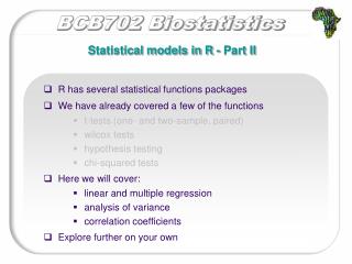
Statistical tests in R Just some examples: > t.test() > pairwise.t.test() > chisq.test() > fisher.test() > ks.test() > …
One sample t-test >data(ChickWeight) > t.test(ChickWeight[, 1], mu = 100) One Sample t-test data: ChickWeight[, 1] t = 7.3805, df = 577, p-value = 5.529e-13 alternative hypothesis: true mean is not equal to 100 95 percent confidence interval: 116.0121 127.6246 sample estimates: mean of x 121.8183
Two sample t-test > t.test(ChickWeight$weight[ChickWeight$Diet == "1"], + ChickWeight$weight[ChickWeight$Diet =="2"]) Welch Two Sample t-test data: ChickWeight$weight[ChickWeight$Diet == "1"] and ChickWeight$weight[ChickWeight$Diet == "2"] t = -2.6378, df = 201.384, p-value = 0.008995 alternative hypothesis: true difference in means is not equal to 0 95 percent confidence interval: -34.899942 -5.042482 sample estimates: mean of x mean of y 102.6455 122.6167
residual error dependent variable intercept independent variable regression coefficient Linear Regression Models Using the methods of least squares, we can derive the following estimators: Our goal is to test the hypothesis: We can do this with a T test: under the null hypothesis, this follows a T distribution with (n-1) df.
Installing ISwR Package Please install the ISwR package on your computer. This package contains all the data sets used in Peter Dalgaard's book Introductory Statistics with R. To load the package into your current R session: > library(ISwR) To find out more information, including what objects are contained in a package: > library(help=ISwR)
Example Dataset tlc We'll be using the dataset tlc that exists in ISwR package. To load this dataset: > data(tlc) # tlc = total lung capacity What kind of object is tlc? > class(tlc) To learn about this dataset: > help(tlc) By using the attach command, we release the columns of the data.frame into the workspace. > attach(tlc) > age
Linear Regression with lm Is there a linear relationship between height and Total Lung Capacity (TLC)? > lmObject <- lm(tlc ~ height, data=tlc) What kind of object is lmObject? > class(lmObject) The model object represents an object that encapsulates the results of a model fit. The desired quantities can be obtained using extractor functions. A basic extractor function is summary: > summary(lmObject)
Interpreting the Output from lm Stores the call to the lm function. Handy for keeping track of what model you fit. Call:... Summary stats of the residuals from the model. Recall: residuals should follow approximately a standard Normal distribution if the model is a good fit. Residuals:... Coefficients:... Estimates from the model. Standard error. T statistics. P-value. Residual standard error:... Residual variance Plug in estimates, to get RSE:
Interpreting the Output from lm Pearson correlation coefficient2 of y, x (e.g. tlc, height). Do cor(tlc[,4], height))^2 to check. Multiple R-squared:... Adjust R-squared:... F statistic: This is the F test that the regression coefficient is zero.
Visualizing Our Fitted Model So what does it really mean, to have fit a linear model of TLC and height? Plot the data: > TLC <- tlc[,4] > plot(height, TLC) Add the regression line we fit with our model: > abline(lmObject)
Values Fitted by the Linear Model Retrieve the fitted values using the extractor function fitted: > fitted(lmObject) Convince yourself that these are the points that fall on the line we just made in the previous plot. > plot(height, TLC) > abline(lmObject) > points(height, fitted(lmObject), pch=20, col="red") To grab the residual values: > resid(lmObject)
Eyeballing Good Fit We can use the information from the residuals and fitted values to create plots to see how good our model fit is. > plot(height, TLC) > abline(lmObject) Use the segments function to draw vertical lines from the fitted values to the real data values. > segments(height, fitted(lmObject), height, TLC) We can also take a look at the residuals. > plot(height, resid(lmObject)) And use a QQ plot to see if the residuals are normally distributed. > qqnorm(resid(lmObject)) > qqline(resid(lmObject))
Confidence Interval Bands Confidence bands are added to regression lines to reflect the uncertainty about a true parameter that cannot be observed i.e. the true regression coefficient . The more narrow the confidence band is, suggests a well-determined line. Using the predict function without any other input arguments yields the fitted values predicted by the model. > predict(lmObject) To compute the confidence interval bands for the fitted values, you need to specify the interval argument: > predict(lmObject, interval="confidence")
Visualizing Confidence Interval Bands Go ahead and plot these values: > pp <- predict(lmObject, interval="confidence") > plot(height, pp[,1], type="l", ylim=range(pp)) > lines(height, pp[,2], col="red", lwd=3) > lines(height, pp[,3], col="blue", lwd=3) What's the problem?
Predicting on New Data Our problem will be solved if height was ordered sequentially. One solution: predict fitted values on new (ordered) height values. Create a sequence of numbers that go from min(height) to max(height) approximately. > range(height) > new <- data.frame(height = seq(from=120, to=200, by=2)) Compute new predictions: > pp.new <- predict(lmObject, new, interval="confidence")
Plotting Confidence Interval Bands Now we can make the plot. First the fitted values: > plot(new$height, pp.new[,1], type="l") Then the upper interval band: > lines(new$height, pp.new[,2], col="red", lwd=2) Finally the lower interval band: > lines(new$height, pp.new[,3], col="blue", lwd=2)
Prediction Interval Bands Prediction interval bands reflect the uncertainty about future observations. Prediction bands are generally wider than the confidence interval bands. > predict(lmObject, interval="prediction") Plot the fitted data with the prediction interval bands and confidence interval bands superimposed. > pp.pred <- predict(lmObject, new, interval="prediction") > pp.conf <- predict(lmObject, new, interval="confidence")
Visualizing Fitted Values, Prediction and Confidence Bands Note: instead of using lines individually, we can also use the function matlines which plots columns of a matrix. > help(matlines) > plot(new$height, pp.pred[,1], ylim=range(pp.pred, pp.conf)) Add the prediction bands: > matlines(new$height, pp.pred[,-1], type=c("l", "l"), lwd=c(3,3), col=c("red", "blue"), lty=c(1,1)) Add the confidence bands: > matlines(new$height, pp.conf[,-1], type=c("l", "l"), lwd=c(3,3), col=c("red", "blue"), lty=c(2,2))
ANOVA Models G levels The (one-way) ANOVA model generalizes linear regression. • One factor that has G levels. • For each level we have J replicates. i = 1 i = 2 … i = G j = 1 ANOVA Model: … J replicates j = J
G levels i = 1 i = 2 … i = G j = 1 … J replicates j = J Total variation: Analysis of Variance Models ANOVA is all about splitting variation up. Variation between groups: Variation within groups:
ANOVA Models Question: is there a significant relationship between our factor A and the response variable Y? If yes, then ideally the variation within groups should be small. The variation between groups should be large. Variation between groups: B = # levels Variation within groups: W = n - B Our test statistic: General idea: Under the null hypothesis that the factor A has no effect: F = 1. Large values of F indicate the factor is significant.
ANOVA Example Let's use a different dataset: > library(MASS) > data(ChickWeight) > attach(ChickWeight) The factor Diet has 4 levels. > levels(Diet) > anova(lm(weight ~ Diet, data=ChickWeight)) Analysis of Variance Table Response: weight Df Sum Sq Mean Sq F value Pr(>F) Diet 3 155863 51954 10.81 6.433e-07 Residuals 574 2758693 4806
Two-way ANOVA We can fit a two-way ANOVA: > anova(lm(weight ~ Diet + Chick, data=ChickWeight)) Analysis of Variance Table Response: weight Df Sum Sq Mean Sq F value Pr(>F) Diet 3 155863 51954 11.5045 2.571e-07 Chick 46 374243 8136 1.8015 0.001359 Residuals 528 2384450 4516 The interpretation of the model output is sequential, from the bottom to the top. This line tests the model: weight ~ Diet + Chick This line tests the model: weight ~ Diet vs weight ~ Diet + Chick.
Multiple Linear Regression • Multiple explanatory variables to explain a response variable. • Can I explain the values of the response variable by the levels of the explanatory variables? • Do I need all explanatory variables to explain the response variable?
Specifying Models In R we use model formula to specify the model we want to fit to our data. y ~ x Simple Linear Regression y ~ x – 1 Simple Linear Regression without the intercept (line goes through origin) y ~ x1 + x2 + x3 Multiple Regression y ~ x + I(x^2) Quadratic Regression log(y) ~ x1 + x2 Multiple Regression of Transformed Variable For factors A, B: y ~ A 1-way ANOVA y ~ A + B 2-way ANOVA y ~ A*B 2-way ANOVA + interaction term
Fit multiple regression model to a data.frame > ##Get data.frame > cfseal <- read.table("cfseal.txt", header=T, + sep="\t") > heart.log <- log(cfseal$heart) > cfseal.log <- cfseal > cfseal.log[,1] <- heart.log > colnames(cfseal.log)[1] <- "heart.log" > ##Fit model > seal.lm <- lm(heart.log ~ ., data=cfseal.log)
Update models and model selection Some handy functions to know about: new.model <- update(old.model, new.formula) Model Selection functions available in the MASS package drop1, dropterm add1, addterm step, stepAIC Similarly, anova(modObj, test="Chisq")
Generalized Linear Models Linear regression models hinge on the assumption that the response variable follows a Normal distribution. Generalized linear models are able to handle non-Normal response variables and transformations to linearity.
Logistic Regression When faced with a binary response Y = (0,1), we use logistic regression. where Logit
Problem 2 – Logistic Regression Read in the anaesthetic data set, data file: anaesthetic.txt. Covariates: move binary numeric vector for patient movement (1 = movement, 0 = no movement) conc anaethestic concentration Goal: estimate how the concentration of movement varies with increasing concentration of the anesthetic agent.
Fit the Logistic Regression Model > anes.logit <- glm(move ~ conc, family=binomial(link=logit), data=anesthetic) The output summary looks like this: > summary(anes.logit) Coefficients: Estimate Std. Error z value Pr(>|z|) (Intercept) 6.469 2.418 2.675 0.00748 ** conc -5.567 2.044 -2.724 0.00645 ** Estimates of P(Y=1) are given by: > fitted.values(anes.logit)
Estimating Log Odds Ratio To get back the log odds ratio > anes.logit$linear.predictors > plot(anesthetic$conc, anes.logit$linear.predictors) > abline(coefficients(anes.logit)) Looks like the odds of not moving increase significantly when you increase the concentration of the anesthetic agent beyond 0.8.
Problem 3 – Multiple Logistic Regression Read in data set birthwt.txt. We fit a logistic regression using the glm function and using the binomial family.
Problem 4 - Poisson Regression Poisson regression is often used for the analysis of count data or the calculation of rates associated with a rare event or disease. Example: schooldata.csv. We can fit the Poisson regression model using the glm function and the poisson family.
Survival Analysis library(survival) Example: aml leukemia data Kaplan-Meier curve fit1 <- survfit(Surv(aml$time[1:11],aml$status[1:11])~1) summary(fit1) plot(fit1) Log-rank test survdiff(Surv(time, status)~x, data=aml)
Survival analysis > cp <- coxph(Surv(aml$time, + aml$status)~x,data=aml) > > summary(cp) > > plot(survfit(Surv(aml$time,aml$status)~x, + data=aml),col=c("red","green"),lwd=2)