Download
1 / 63
660 likes | 936 Vues
Simultaneous EEG and f MRI Acquisition. Mark Cohen UCLA Brain Mapping Center. Outline. Motivation: It’s hard , why bother ? Problems and Solutions Early Results. fMRI-EEG. Levels of Understanding. fMRI functional nuclei or processing centers. Fiber Tracing regional connectivity.

E N D
Simultaneous EEG and fMRI Acquisition Mark Cohen UCLA Brain Mapping Center
Outline • Motivation: It’s hard, why bother? • Problems and Solutions • Early Results
fMRI-EEG Levels of Understanding fMRIfunctional nuclei or processing centers Fiber Tracingregional connectivity EEG & Autoradiographycell assemblies Multi-unit Recordinglocal circuits: columns, retina… Single Unit Electrophysiologyaction potentials, chemomodulation Crystallography, Chromatography (etc…)transmitters, ion channels, membrane proteins
- - - + - + + + + + Presumed Origin of the EEG Skin Bone CSF
Many Neurons are Not “Seen” by EEG Skin Bone Bone CSF
General Limitations in EEG Localization • Deeper Sources Show Weaker Signals • Magnitude Depends on Dipole Orientation • Magnitude Depends on Temporal Synchrony • Magnitude Depends on Spatial Coherence • Conductivity of Body Tissues (CSF, scalp) Blur the Scalp Potentials
EEG Source Localization after Massoud Akhtari • High resolution raw data • High temporal resolution EEG • High spatial resolution imaging • Computational Capacity • Accurate Mathematical Models • Maxwell’s Equation forward model • Non-singular Inversion • Accurate Physiological Parameters • Conductivity of all relevant tissues ≥10 kHz ≤ 1 mm
? ? ? ? ? EEG Source Localization after Massoud Akhtari
The Scalp Waveform is Distorted MEG ECoG
10 100 1000 Hz R The observed spectrally-dependent conductivity implies not only Resistive elements, but both Capacitive and Inductive energy storage. C L R Such elements result in substantial phase lags that can alter the dipole localization by several millimeters. Akhtari, unpublished the Brain and Skull Exhibit Complex Impedance p/4 0 phase Conductivity,s 10 100 1000 Hz -p/4 -p/2
How does BOLD relate to neural firing? • Energy Demands in Transmission • Pre-synaptic: • Transmitter Synthesis • Exocytosis • Transmitter re-uptake • Post-Synaptic • Maintenance of membrane potential after ion leakage • Excitatory: Removal of Sodium (Na/K pump) • Inhibitory: ???
Red and Green Spikes Seizure Activity Spreads from an Irritative Zone • Hypotheses: • Initial Event is Energetically Costly • Spreading Depolarization is Not EEG-correlated fMRI, New York
Spike-Triggered fMRI R R • Complex partial seizures, rare generalization • EEG: generalized interictal discharges, some with left temporal onset • MRI: normal • Complex partial seizures, occasional generalization • EEG: multifocal and generalized interictal discharges • MRI: symmetric subependymal heterotopias Warach, et al. (1996)
Project Goals • Unaltered MR Image Quality • Diagnostic Quality EEG During functional MRI: Artifact Free Dense Array of Channels • Tomographic Correlation of Scalp Electrical Activity • Amplifiers Suitable for Single Units • Subject Safety
RF Noise Signal Losses Artifacts - MRI Magnetic Field Distortion Non-magnetic material such as Silver • Careful Lead Dress • Eliminate RF Loops • Properly-shielded Amplifiers • Softened Logic Pulses
+ – Inductive Pickup by EEG leads Imaging Field Gradients Ballistocardiogram
Ballistocardiogram Subtraction QRS EKG A B A-B 0 1 2 3 time (sec) Goldman, et al., Clinical Neurophysiology, 2000
ECG correction • Fourier detection of nominal heart rate • Bootstrap detection of QRS based on template • Adaptively create template of complete ECG • Outlier and error monitoring • Further detection based on statistical correlation peak • Continuous adaptation of nominal HR and waveforms
Artifact N S Sk k=1 – N S + EEGk Approach to MR Artifact Removal Sk=EEGk+Artifact This approach requires that: • EEGk and Artifact are uncorrelated • EEGk and Artifact add linearly • Artifact is identical at each time (k)
EEG Lead Configuration Minimized Current Induction: • High Impedance Carbon Fiber Leads • Reduced loop area • Self canceling currents A B C Hard-Wired Bipolar Montage: • Dual lead electrodes • Twisted lead pairs • Local differential amplifiers – – + + Goldman, et al., Clinical Neurophysiology, 2000 Patent Applied For
EEG Physical Apparatus Goldman, et al., Clinical Neurophysiology, 2000 Patent Applied For
Twisted Lead Noise Reduction no scan scan untwisted fp2f8 c4p4 twisted fp1f7 c3p3 0 1 2 time (sec) Goldman, et al., Clinical Neurophysiology, 2000
1 sec Amplifier Recovery
2 Hz + OUT – 150 mV 150 mV IN OUT DC offset 1 2 1 2 Time (sec) Time (sec) Receiver Saturation IN
Differential Amp Twisted Range detect Pair Leads 73 + 58 1 – 3 High Pass 72 64 Isolation Low Pass Barrier Shield Driver + – EEG Functional Block Diagram Patent Applied For
10 µV 0 0.1 0.2 0.3 0 5 10 15 20 25 After DC Offset control & Low Pass Filter 100 µV sec Gradient Artifacts are not eliminated completely by analog means. msec
100 µV 10 µV 5 10 15 20 25 0 Fast Sampling is NOT enough Raw Signal After Subtraction of Averaged Artifact Sampling rate: 10 kHz 0 0.1 0.2 0.3 0.4 0.5 0.6 After Subtraction of Averaged Artifact 0 5 10 15 20 25
e j t Residual Errors • …where: ƒ is the frequency of the artifact • is the phase error, equal to 2πf0/fs, • - f0 is the EPI readout frequency and • - fs is the sampling frequency. At high sampling frequency (small j) the error, e, is linearly proportional to the sampling frequency
Triggered Adaptive Correction Differential Amplification DC Offset Correction Analog Filter Digitization Averaging + Fc=100 Hz EEG ≥200 s/s 16 bits + S – – – + – Trigger once per tr + Corrected EEG Patent Applied For
Uncorrected Average N=30 Corrected Sampled Gradient Drive Current Corrected X 5 0 0.5 1 1.5 2 2.5 3 Time (seconds)
50 µV EEG Correction During Continuous Scan tr = 2.5 s te = 30 ms 20X20 cm 15 slices
MRI-Compatible EEG System Design 64 Channel Local Amplifier EEG Leads USB over Optical Fiber Analog to Digital Convertor & Digital Signal Processor EEG Display Within the MR scanner (anonymized subject)
State Measurements • EEG may be the best available measure of state: • Sleep • Attentiveness • Arousal • Responsiveness
EEG during Sleep (corrected) fp2-f8 fp2-f8 fp8-t4 fp8-t4 t4-t6 t4-t6 t6-o2 t6-o2 fp2-f4 fp2-f4 f4-c4 f4-c4 c4-p4 c4-p4 p4-o2 p4-o2
UCLA: Simultaneous fMRI & Epileptiform EEG fp2-f8 f8-t4 t4-t6 t6-o2 fp1-t7 t7-t3 t3-t5 t5-o1 fp2-f4 f4-c4 c4-p4 p4-o2 fp1-f3 f3-c3 c3-p3 p3-O1 1 sec
EEG Spectral Content Goldman, et al., Clinical Neurophysiology, 2000
Linear Systems Approach • Linear • Time-Invariant • (LTI) System x(t) y(t) = ƒ[x(t)] ƒ(A + B) = ƒ(A) + ƒ(B) If h(t) is the response to an impulse:
Response Latency vs. Stimulus DurationAverage of 10 recordings Stimulus Onset 100 ms flash Signal 17 ms flash 1 sec flash Data courtesy R. Savoy / Mass. General Hospital
Brain Impulse Response Light Flash 50 • • • • • 40 • Raw Data from R. Savoy • 30 MR Signal (a.u.) • • 20 • • 10 • • • • • • • • • • • • • • • • • 0 • • • -10 0 2 4 6 8 10 12 14 16 Time (seconds)
spectral power in the alpha band 1.6 predicted BOLD response 1.4 1.2 1 Average Power (µV2) 0.8 0.6 0.4 0.2 0 0 25 50 75 100 125 150 175 200 225 250 0 1 2 3 4 time (sec) time (minutes) Alpha Mapping
25 20 15 10 5 15 20 25 Gamma Spectral Time Course Theta
EEG spectral fMRI + 0.6 ± 0.3 – 0.6 Goldman, et al., NeuroReport, 2003 Patent Applied For
Q&A Q: Do the spectral bands adequately describe the EEG? Q: Is the forward convolution model valid? Q: What is the explanatory power of the data? A: Ask a mathematician.
S(NdX NwX Nt) is a three dimensional matrix, d are the electrode pairs, w is frequency and t is time. PARAFAC a channel k Nk b k = S EEG S time ftd k c k frequency Each atom, k, is the trilinear combination of f, t and d F. Miwakeichi, et al., NeuroImage 22, 2004
Find: that explain S with minimal error. PARAFAC a A channel k Nk b k = = S EEG S B time ftd k c k C frequency The “corcondia”(=core consistency diagnostic) constraint determines Nk. F. Miwakeichi, et al., NeuroImage 22, 2004
PARAFAC applied to SITE data 0.4 theta alpha gamma 0.3 Rel. Energy 0.2 0.1 0.1 0 10 20 30 40 50 Frequency (Hz)
Trilinear Partial Least Squares a A channel k b = S = k EEG S B time ftd k c k C frequency Maximize covariance u = S = k fMRI f U time st v k k V voxel E. Martinez-Montes, et al., in preparation, 2003