Probability Concepts and Applications
Probability Concepts and Applications. Chapter 2. To accompany Quantitative Analysis for Management , Tenth Edition , by Render, Stair, and Hanna Power Point slides created by Jeff Heyl. © 2009 Prentice-Hall, Inc. . Learning Objectives.

Probability Concepts and Applications
E N D
Presentation Transcript
Probability Concepts and Applications Chapter 2 To accompanyQuantitative Analysis for Management, Tenth Edition,by Render, Stair, and Hanna Power Point slides created by Jeff Heyl © 2009 Prentice-Hall, Inc.
Learning Objectives After completing this chapter, students will be able to: • Understand the basic foundations of probability analysis • Describe statistically dependent and independent events • Use Bayes’ theorem to establish posterior probabilities • Describe and provide examples of both discrete and continuous random variables • Explain the difference between discrete and continuous probability distributions • Calculate expected values and variances and use the normal table
Chapter Outline 2.1Introduction 2.2Fundamental Concepts 2.3Mutually Exclusive and Collectively Exhaustive Events 2.4Statistically Independent Events 2.5Statistically Dependent Events 2.6Revising Probabilities with Bayes’ Theorem 2.7Further Probability Revisions
Chapter Outline 2.8 Random Variables 2.9 Probability Distributions 2.10 The Binomial Distribution 2.11 The Normal Distribution 2.12 The F Distribution 2.13 The Exponential Distribution 2.14 The Poisson Distribution
Introduction • Life is uncertain, we are not sure what the future will bring • Risk and probability is a part of our daily lives • Probability is a numerical statement about the likelihood that an event will occur
Fundamental Concepts • The probability, P, of any event or state of nature occurring is greater than or equal to 0 and less than or equal to 1. That is: 0 P (event) 1 • The sum of the simple probabilities for all possible outcomes of an activity must equal 1
Diversey Paint Example • Demand for white latex paint at Diversey Paint and Supply has always been either 0, 1, 2, 3, or 4 gallons per day • Over the past 200 days, the owner has observed the following frequencies of demand
Diversey Paint Example • Demand for white latex paint at Diversey Paint and Supply has always been either 0, 1, 2, 3, or 4 gallons per day • Over the past 200 days, the owner has observed the following frequencies of demand Notice the individual probabilities are all between 0 and 1 0 ≤ P (event) ≤ 1 And the total of all event probabilities equals 1 ∑ P (event) = 1.00
1 2 Number of occurrences of the event Total number of trials or outcomes Number of ways of getting a head Number of possible outcomes (head or tail) P (event) = P (head) = Types of Probability Determiningobjective probability • Relative frequency • Typically based on historical data • Classical or logical method • Logically determine probabilities without trials
Types of Probability Subjective probability is based on the experience and judgment of the person making the estimate • Opinion polls • Judgment of experts • Delphi method • Other methods
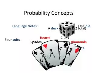
Mutually Exclusive Events Events are said to be mutually exclusive if only one of the events can occur on any one trial • Tossing a coin will result in eithera head or a tail • Rolling a die will result in only one of six possible outcomes
Collectively Exhaustive Events Events are said to be collectively exhaustiveif the list of outcomes includes every possible outcome • Both heads and tails as possible outcomes of coin flips • All six possible outcomes of the roll of a die
Drawing a Card Draw one card from a deck of 52 playing cards P (drawing a 7) = 4/52 = 1/13 P (drawing a heart) = 13/52 = 1/4 • These two events are not mutually exclusive since a 7 of hearts can be drawn • These two events are not collectively exhaustive since there are other cards in the deck besides 7s and hearts
Adding Mutually Exclusive Events • We often want to know whether one or a second event will occur • When two events are mutually exclusive, the law of addition is – P (event A or event B) = P (event A) + P (event B) P (spade or club) = P (spade) + P (club) = 13/52 + 13/52 = 26/52 = 1/2 = 0.50 = 50%
Adding Not Mutually Exclusive Events • The equation must be modified to account for double counting • The probability is reduced by subtracting the chance of both events occurring together P (event A or event B) = P (event A) + P (event B) –P (event Aand event B bothoccurring) P (A or B) = P (A) + P (B) –P (A and B) P(five or diamond) =P(five) + P(diamond) – P(five and diamond) = 4/52 + 13/52 – 1/52 = 16/52 = 4/13
P (A and B) P (A) P (B) P (A) P (B) Events that are mutually exclusive Events that are not mutually exclusive P (A or B) = P (A) + P (B) P (A or B) = P (A) + P (B)–P (A and B) Figure 2.1 Figure 2.2 Venn Diagrams
Statistically Independent Events Events may be either independent or dependent • For independent events, the occurrence of one event has no effect on the probability of occurrence of the second event
Dependent events Independent events Dependent events Independent events Which Sets of Events Are Independent?
Three Types of Probabilities • Marginal (or simple) probability is just the probability of an event occurring P (A) • Joint probability is the probability of two or more events occurring and is the product of their marginal probabilities for independent events P (AB) = P (A) x P (B) • Conditional probability is the probability of event B given that event A has occurred P (B | A) = P (B) • Or the probability of event A given that event B has occurred P (A | B) = P (A)
Joint Probability Example The probability of tossing a 6 on the first roll of the die and a 2 on the second roll P (6 on first and 2 on second) = P (tossing a 6) x P (tossing a 2) = 1/6 x 1/6 = 1/36 = 0.028
A black ball drawn on first draw P (B) = 0.30 (a marginal probability) Two green balls drawn P (GG) = P (G) x P (G) = 0.7 x 0.7 = 0.49(a joint probability for two independent events) Independent Events • A bucket contains 3 black balls and 7 green balls • We draw a ball from the bucket, replace it, and draw a second ball
A black ball drawn on second draw if the first draw is green P (B | G) = P (B) = 0.30 (a conditional probability but equal to the marginal because the two draws are independent events) A green ball is drawn on the second if the first draw was green P (G | G) = P (G) = 0.70(a conditional probability as in event 3) Independent Events • A bucket contains 3 black balls and 7 green balls • We draw a ball from the bucket, replace it, and draw a second ball
Calculating conditional probabilities is slightly more complicated. The probability of event A given that event B has occurred is P (AB) P (B) P (A | B) = Statistically Dependent Events The marginal probability of an event occurring is computed the same P (A) The formula for the joint probability of two events is P (AB) = P (B | A) P (A)
When Events Are Dependent • Assume that we have an urn containing 10 balls of the following descriptions • 4 are white (W) and lettered (L) • 2 are white (W) and numbered (N) • 3 are yellow (Y) and lettered (L) • 1 is yellow (Y) and numbered (N) P (WL) = 4/10 = 0.4 P (YL) = 3/10 = 0.3 P(WN) = 2/10 = 0.2 P (YN) = 1/10 = 0.1 P (W) = 6/10 = 0.6 P (L) = 7/10 = 0.7 P (Y) = 4/10 = 0.4 P (N) = 3/10 = 0.3
4 10 1 10 3 10 2 10 4 balls White (W) and Lettered (L) Probability (WL) = Probability (WN) = 2 balls White (W) and Numbered (N) Urn contains 10 balls Probability (YL) = 3 balls Yellow (Y) and Lettered (L) Probability (YN) = 1 ball Yellow (Y) and Numbered (N) When Events Are Dependent Figure 2.3
The conditional probability that the ball drawn is lettered, given that it is yellow, is P (L| Y) = = = 0.75 P (YL) P (Y) Verify P (YL) using the joint probability formula P (YL) = P (L| Y) x P (Y) = (0.75)(0.4) = 0.3 0.3 0.4 When Events Are Dependent
P (MT) = P (T | M) x P (M) = (0.70)(0.40) = 0.28 Joint Probabilities for Dependent Events • If the stock market reaches 12,500 point by January, there is a 70% probability that Tubeless Electronics will go up • There is a 40% chance the stock market will reach 12,500 • Let M represent the event of the stock market reaching 12,500 and let T be the event that Tubeless goes up in value
Prior Probabilities Posterior Probabilities Bayes’ Process New Information Revising Probabilities with Bayes’ Theorem Bayes’ theorem is used to incorporate additional information and help create posterior probabilities Figure 2.4
A cup contains two dice identical in appearance but one is fair (unbiased), the other is loaded (biased) The probability of rolling a 3 on the fair die is 1/6 or 0.166 The probability of tossing the same number on the loaded die is 0.60 We select one by chance, toss it, and get a result of a 3 What is the probability that the die rolled was fair? What is the probability that the loaded die was rolled? Posterior Probabilities
We know the probability of the die being fair or loaded is P (fair) = 0.50 P (loaded) = 0.50 And that P (3 | fair) = 0.166 P (3 | loaded) = 0.60 We compute the probabilities of P (3 and fair) and P (3 and loaded) P (3 and fair) = P (3 | fair) x P (fair) = (0.166)(0.50) = 0.083 P (3 and loaded) = P (3 | loaded) x P (loaded) = (0.60)(0.50) = 0.300 Posterior Probabilities
We know the probability of the die being fair or loaded is P (fair) = 0.50 P (loaded) = 0.50 And that P (3 | fair) = 0.166 P (3 | loaded) = 0.60 The sum of these probabilities gives us the unconditional probability of tossing a 3 P (3) = 0.083 + 0.300 = 0.383 We compute the probabilities of P (3 and fair) and P (3 and loaded) P (3 and fair) = P (3 | fair) x P (fair) = (0.166)(0.50) = 0.083 P (3 and loaded) = P (3 | loaded) x P (loaded) = (0.60)(0.50) = 0.300 Posterior Probabilities
If a 3 does occur, the probability that the die rolled was the fair one is 0.083 0.383 P (fair and 3) P (3) P (fair | 3) = = = 0.22 The probability that the die was loaded is 0.300 0.383 P (loaded and 3) P (3) P (loaded | 3) = = = 0.78 Posterior Probabilities • These are the revised or posteriorprobabilities for the next roll of the die • We use these to revise our prior probability estimates
Bayes Calculations Given event B has occurred Table 2.2 Given a 3 was rolled Table 2.3
where the complement of the event ; for example, if is the event “fair die”, then is “loaded die” ¢ = A General Form of Bayes’ Theorem We can compute revised probabilities more directly by using
If we replace with “fair die” Replace with “loaded die Replace with “3 rolled” We get General Form of Bayes’ Theorem This is basically what we did in the previous example
Further Probability Revisions • We can obtain additional information by performing the experiment a second time • If you can afford it, perform experiments several times We roll the die again and again get a 3
Further Probability Revisions • We can obtain additional information by performing the experiment a second time • If you can afford it, perform experiments several times We roll the die again and again get a 3
Further Probability Revisions • We can obtain additional information by performing the experiment a second time • If you can afford it, perform experiments several times We roll the die again and again get a 3
Further Probability Revisions After the first roll of the die – probability the die is fair = 0.22 probability the die is loaded = 0.78 After the second roll of the die – probability the die is fair = 0.067 probability the die is loaded = 0.933
Random Variables Discrete random variables can assume only a finite or limited set of values Continuous random variables can assume any one of an infinite set of values A random variable assigns a real number to every possible outcome or event in an experiment X = number of refrigerators sold during the day
Random Variables – Numbers Table 2.4
Random Variables – Not Numbers Table 2.5
5. Strongly agree 4. Agree 3. Neutral 2. Disagree 1. Strongly disagree Probability Distribution of a Discrete Random Variable Selecting the right probability distribution is important • For discrete random variables a probability is assigned to each event Dr. Shannon asked students to respond to the statement, “The textbook was well written and helped me acquire the necessary information.”
Probability Distribution of a Discrete Random Variable Table 2.6 • Distribution follows all three rules • Events are mutually exclusive and collectively exhaustive • Individual probability values are between 0 and 1 • Total of all probability values equals 1
0.4 – 0.3 – 0.2 – 0.1 – 0 – P (X) | | | | | | 1 2 3 4 5 X Probability Distribution for Dr. Shannon’s Class Figure 2.5
0.4 – 0.3 – 0.2 – 0.1 – 0 – Central tendency of the distribution is the mean or expected value Amount of variability or spread is the variance P (X) | | | | | | 1 2 3 4 5 X Probability Distribution for Dr. Shannon’s Class Figure 2.5
where = random variable’s possible values = probability of each of the random variable’s possible values = summation sign indicating we are adding all n possible values = expected value or mean of the random sample Expected Value of a Discrete Probability Distribution The expected value is a measure of the central tendency of the distribution and is a weighted average of the values of the random variable
where = random variable’s possible values = expected value of the random variable = difference between each value of the random variable and the expected mean = probability of each possible value of the random sample Variance of a Discrete Probability Distribution For a discrete probability distribution the variance can be computed by