Chapter 05 Constraint Satisfaction Problems

1. Chapter 05Constraint Satisfaction Problems Artificial Intelligence Section 1 – 3

2. Outline • Constraint Satisfaction Problems (CSP) • Backtracking search for CSPs • Local search for CSPs

3. Review • Standard search problem: • Problems can be solved by searching in a space of states. • Evaluate these states by domain-specific and • test to see whether they are goal states. • From the point of view of the search algorithm, • each state is atomic, or indivisible – a “black box” with no internal structure. • state is a "black box“ – any data structure that supports successor function, heuristic function, and goal test

4. Feature Vectors – for our understanding: • • We have • A set of k variables (or features) • Each variable has a domain of different values. • A state is specified by an assignment of a value for each variable. • height = {short, average, tall}, • weight = {light, average, heavy} • A partial state is specified by an assignment of a value to some of the variables.

5. Example: 8--‐Puzzle Missionaries and Cannibals Romania Map Water Jugs Problem N-queens Problem • Variables: 9 variables Cell1,1, Cell1,2, …, Cell3,3 • Values: {‘B’, 1, 2, …, 8} • State: Each “Celli,j” variable specifies what is in that position of the tile. • If we specify a value for each cell we have completely specified a state. • This is only one of many ways to specify the state.

6. Constraint Satisfaction Problems • Notice that in these problems some settings of the variables are illegal. • In the 8 puzzle each variable must have a distinct value (same tile can’t be in two places) • in the 8-puzzle, the feature vector satisfying the goal is given. We care about the sequence of moves needed to move the tiles into that configuration

7. Constraint Satisfaction Problems • In general, • In many of the CSPs, we do not care about the sequence of moves needed to get to a goal state. • We only care about finding a feature vector (a setting of the variables) that satisfies the goal. • A setting of the variables that satisfies some constraints.

9. Constraint satisfaction problems (CSPs) • CSP: • state is defined by variablesXi with values from domainDi • goal test is a set of constraints specifying allowable combinations of values for subsets of variables • Simple example of a formal representation language • Allows useful general-purpose algorithms with more power than standard search algorithms

10. CSP - Constraint satisfaction problem: • Use a factored representation for each state: • A set of variables, each of which has a value. • A set of constraints the specify allowable combinations of values. • A constraint satisfaction problem is solved when each variable has a value that satisfies all the constraints on the variable. • From the point of view of the CSP search algorithm, • Allow to eliminate large portions of the search space all at once by identifying variable/value combination that violate the constraints. • Take advantage of the structure of states and use general-purpose rather problem-specific heuristics for finding the solution of complex problems efficiently.

11. Formalization of a Constraint satisfaction problem (CSP): • A CSP consists of X, D, and C: • A set X of variables Xi, X = {X1, …, Xn }. • A set D of domainsDi, D = {D1, …, Dn }, one for each variable. • Each domain Di consists of a set of allowable values, {v1, …, vk }, for each variable Xi. Di[Xi] = {v1, …, vk }. • A set C of constraints C = {C1,…, Cm}, that specify allowable combinations of values. • …

12. Formalization of a Constraint satisfaction problem (CSP): • A CSP consists of X, D, and C: • … • A set C of constraints C = {C1,…, Cm}, that specify allowable combinations of values. • Each constraint C has a set of variables it is over, called its scope • E.g., C(X1, X2, X4) is a constraint over the variables X1, X2, and X4. Its scope is {X1, X2, X4}. • Each constraint Ci consists of a pair <scope, rel>, where scope is a tuple of variables that participate in the constraint andrelis a relation that defines the values that those variables can take on.

13. Formalization of a Constraint satisfaction problem (CSP): • A relation can be represented as • an explicit list of all tuples of values that satisfy the constraint, or • an abstract relation that supports two operations: • testing if a tuple is a member of the relation and • enumerating the members of the relation. • For example, if both X1 and X2 are the domain {A, B}, then the constraint saying the two variables must have different values can be written as • < (X1, X2), [(A, B), (B, A)] > or • < (X1, X2), X1 X2 >. • Given an assignment to its variables, the constraint returns: • True—this assignment satisfies the constraint • False—this assignment falsifies the constraint.

14. Formalization of a Constraint satisfaction problem (CSP): • We can specify the constraint with a table • C(X1, X2, X4) is a constraint over the variables X1, X2, and X4 where C(X1, X2, X4) with D1 [X1] = {1,2,3} and D2 [X2] = D4 [X4] = {1, 2}

15. Formalization of a Constraint satisfaction problem (CSP): Often we can specify the constraint more compactly with an expression: C(X1, X2, X4) = ( X1 = X2 + X4 )

16. Formalization of a Constraint satisfaction problem (CSP): • Unary Constraints (over one variable) • e.g. C(X): X = 2; • C(Y): Y > 5 • Binary Constraints (over two variables) • e.g. C(X,Y): X + Y < 6 • Higher-order constraints: over 3 or more variables.

17. Solving Constraint satisfaction problems (CSPs): • Because CSPs do not require finding a paths (to a goal), it is best solved by a specialized version of depth-first search. • Key intuitions: • We can build up to a solution by searching through the space of partial assignments. • Does not matter about order in which we assign the variables; eventually they all have to be assigned. • We can decide on a suitable value for one variable at a time! • This is the key idea of backtracking search. • If we falsify a constraint during the process of building up a solution, we can immediately reject the current partial assignment: • All extensions of this partial assignment will falsify that constraint, and thus none can be solutions.

18. CSP - Constraint satisfaction problem: • To solve a CSP, we need to define a state space and notion of a solution. • Each state in a CSP is defined by {Xi = vi , Xj = vj, …}, an assignment of values to some or all the variables. • An assignment that does not violate any constraints is called consistent or legal assignment. • A complete assignment is one in which every variable is assigned. • A solution to a CSP is a consistent, complete assignment. • A solutionto a CSP is an assignment of a value to all of the • variables such that every constraint is satisfied. • A CSP is unsatisfiable if no solution exists. • A partial assignment is one that assigns values to only some of the variables.

19. CSP as a Search Problem • A CSP could be viewed as a more traditional search problem • Initial state: empty assignment • Successor function: a value is assigned to any unassigned variable, which does not cause any constraint to return false. • Goal test: the assignment is complete

20. Backtracking Search: The Algorithm BT • BT(Level) • if all variables assigned • PRINT Value of each Variable • RETURN or EXIT (RETURN for more solutions) • (EXIT for only one solution) • X := PickUnassignedVariable() • Assigned[X] := TRUE • for d := each member of Domain[X] (the domain values of X) • Value[X] := d • ConstraintsOK = TRUE • for each constraint C such that • a) X is a variable of C and • b) all other variables of C are assigned: • if C is not satisfied by the set of current assignments: • ConstraintsOK = FALSE • if ConstraintsOk == TRUE: • BT(Level+1) • Assigned[X] := FALSE //UNDO as we have tried all of X’s values • return

21. Backtracking Search The root has the empty set of assignments Children of a node are all possible values of some (any) unassigned variable Root { } Xi = a Xi = c Xi = b Search stops descending if the assignments on path to the node violate a constraint Xj = 2 Xj = 1 Subtree

22. Backtracking Search • Heuristics are used to determine • the order in which variables are assigned: • PickUnassignedVariable( ) • the order of values tried for each variable. • The choice of the next variable can vary from branch to branch, e.g., • under the assignment X1 = a we might choose to assign X4 next, while under X1 = b we might choose to assign X5 next. • This “dynamically” chosen variable ordering has a tremendous impact on performance. such as, Q1, Q2, …, Q8 such as, Qi = j

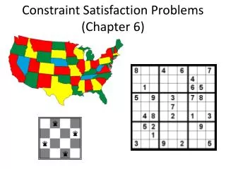
23. Example: N-Queens Place N Queens on an N x N chess board so that no Queen can attack any other Queen.

24. Example: N-Queens • Problem formulation: • N variables (N queens) • N2 values for each variable representing the positions on the chessboard • Value i is ith cell counting from the top left as 1, going left to right, top to bottom. • For example Q1 has a value 1, Q2 has a value 15, Q3 has a value 21, etc.

25. Example: N-Queens Q1 = 1, Q2 = 15, Q3 = 21, Q4 = 32, Q5 = 34, Q6 = 44, Q7 = 54, Q8 = 59

26. Example: N-Queens • This representation has (N2)N states • (different possible assignments in the search space) • For 8-Queens: 648 = 281,474,976,710,656 • Is there a better way to represent the N-queens problem? • We know we cannot place two queens in a single row we can exploit this fact in the choice of the CSP representation

27. Example: N-Queens • Better Modeling: • N variables Qi, one per row. • Value of Qi is the column the Queen in row i is placed; possible values {1, …, N}. • This representation has NN states: • For 8-Queens: 88 = 16,777,216 • The choice of a representation can make the problem solvable or unsolvable!

28. Example: N-Queens Q1 = 1, Q2 = 7, Q3 = 5, Q4 = 8, Q5 = 2, Q6 = 4, Q7 = 6, Q8 = 3

29. Example: N-Queens • Constraints: • Can’t put two Queens in same column • Qi ≠ Qj for all i ≠ j • Diagonal constraints • abs(Qi - Qj) ≠ abs(i - j) • i.e., the difference in the values assigned to Qi and Qj can’t be equal to the difference between i and j.

30. Example: N-Queens Place N Queens on an N x N chess board so that no Queen can attack any other Queen. • Two Qs in same column: • Q1 = Q2= 4, 1 2 • … • Q1 = Q8 = 4, 1 8 • each of which violates • Qi ≠ Qji ≠ j. • Diagonal constraints: • For Q1 = 4, Q5 = 8, i = 1 and j = 5, abs(4 – 8) = abs (1 – 5), which violates • abs(Qi - Qj) ≠ abs(i - j) • Can’t put two Queens in same column • Qi ≠ Qji ≠ j • Diagonal constraints • abs(Qi - Qj) ≠ abs(i - j)

31. Example: N-Queens

32. Example: N-Queens

33. Example: N-Queens Solution

34. Example: N-Queens Backtracking Search Space

35. Example: N-Queens Backtracking Search Space Continue from previous viewgraph Solution

36. Problems with Plain Backtracking • In the backtracking search we won’t detect that a cell has no possible value until all variables of the row/column or the subsquare constraint are assigned. So we have the following situation: • Leads to the idea of constraint propagation Variable has no possible value, but we don’t detect this. Until we try to assign it a value

37. Constraint Propagation • Constraint propagation refers to the technique of “looking ahead” at those unassigned variables in the search . • Try to detect obvious failures: • “Obvious” means things we can test/detect efficiently. • Even if we don’t detect an obvious failure we might be able to eliminate some possible part of the future search. e.g., an example in previous slides.

38. Constraint Propagation • Propagation has to be applied potentially at every node of the search tree, during the search. • Propagation itself is an inference step that needs some resources (such as time and space) • If propagation is slow, this can slow the search down to the point where using propagation for finding a solution will take longer! • There is always a tradeoff between searching fewer nodes in the search, and having a higher nodes/second processing rate. • We will look at two main types of propagation: • Forward Checking & Generalized Arc Consistency

40. Example: Map-Coloring Fig 6.1 (a) The principal states and territories of Australia. The goal is to assign colors to each region either red, green or blue with the constraint that no neighboring regions have the same color. Formulate this as a CSP: Modeling • Variables: X = {WA, NT, Q, NSW, V, SA, T } • Domains:The domain of each variable is the set Di = {red, green, blue} • Constraints: adjacent regions must have different colors • e.g., WA ≠ NT, or (WA,NT) in {(red, green), (red, blue), (green, red), (green, blue), (blue, red), (blue, green)}

41. Example: Map-Coloring Fig 6.1 (a) The principal states and territories of Australia. The task of coloring each region either red, green or blue with the constraint that no neighboring regions have the same color. Formulate this as a CSP: • Variables: X = {WA, NT, Q, NSW, V, SA, T } • Domains: Di = {red, green, blue} • Constraints: C = {<(SA, WA), SA WA>, <(SA, NT), SA NT>, <(SA, Q), SA Q>, <(SA, NSW), SA NSW>, <(SA, V), SA V>, <(WA, NT), WA NT>, <(NT, Q>), NT Q>, <(Q, NSW), Q NSW>, <(NSW, V), NSW V>} • e.g., WA ≠ NT, or (WA,NT) can be fully enumerated in turn as {(red, green), (red, blue), (green, red), (green, blue), (blue, red), (blue, green)} • One of the possible solutions is {WA = red, NT = green, Q = red, NSW = green, V = red, SA = blue, T = red }

42. Example: Map-Coloring • Solutions are complete and consistent assignments, • e.g., WA = red, NT = green, Q = red, NSW = green, V = red, SA = blue, T = green. • complete assignment: every variable is assigned to a value • Consistent assignment: the assignment does not violate any constraints.

43. Constraint graph- Visualize a CSP as a constraint graph • Binary CSP: each constraint relates two variables • Constraint graph: nodes are variables, arcs are constraints • General-purpose CSP methods use the graph structure to speed up search • e.g., Tasmania is an independent subproblem! Fig 6.1(b) The map-coloring problem represented as a constraint graph.

44. Why formulate a problem as a CSP? • A CSP – solvers can be faster than state-space searchers because: • the CSP solver can quickly eliminate large swatches of the search space. • e.g., Once {SA blue} is selected in the Australia problem, then none of the five neighboring variables can take on the value blue. • Without taking advantage of constraint propagation, a search procedure would have to consider 35 = 243 assignments for the five neighboring variables; • with constraint propagation, we never have to consider blue as a value, so we have only 25 = 32 assignments to look at, a reduction of 87%

45. Why formulate a problem as a CSP? • In regular state-space search we can only ask: • Is this specific state a goal? No? What about this one? • With CSPs, once we find out that a partial assignment (assigns values to only some of the variables) is not a solution, • we can immediately discard further refinements of the partial assignment. • With CSPs, we can see • why the assignment is not a solution • which variable violate a constraint So, we can focus attention on the variables that matter. • As a result, many problems that are intractable for regular state-space search can be solved quickly when formulated as a CSP.

47. CSP: Constraint Satisfaction Problems - recall • Set of vars, set of possible values for each vars, and set of • constraints defines a CSP. • A solution to the CSP is an assignment of values to the • variables (i.e., complete) so that all constraints are satisfied • (no “violated constraints.” i.e., consistent) • A CSP is inconsistent if no such solution exists for satisfying the given constraints. • e.g. try to place 9 non-attacking queens on an 8 x 8 • board.

48. CSP: Constraint Satisfaction Problems - recall • Set of variables {X1, X2, …, Xn} • Each variable Xi has a domain Di of possible values • Usually Di is discrete and finite • Set of constraints {C1, C2, …, Cp} • Each constraint Ck involves a subset of variables and • specifies the allowable combinations of values of • these variables • Goal: Assign a value to every variable such that all constraints are satisfied

49. Varieties of CSPs • Discrete variables • finite domains: • n variables, domain size d  O(dn) complete assignments • e.g., Boolean CSPs, including Boolean satisfiability (NP-complete) • infinite domains: • integers, strings, etc. • e.g., job scheduling, variables are start/end days for each job • need a constraint language, e.g., StartJob1 + 5 ≤ StartJob3 • linear constraints solvable, nonlinear undecidable • Continuous variables • e.g., start/end times for Hubble Space Telescope observations • linear constraints solvable in polynomial time by linear programming methods

50. Varieties of constraints • Unary constraints involve a single variable, • e.g., SA ≠ green • Binary constraints involve pairs of variables, • e.g., SA ≠ WA • Higher-order constraints involve 3 or more variables, • e.g., cryptarithmetic column constraints • Preferencesare soft constraints • e.g., redis better than green • often representable by a cost for each variable assignment → constrained optimization problems Knapsacks