Download
1 / 44
440 likes | 542 Vues
Learn about confidence intervals and hypothesis tests for a population mean using t-distributions. Understand the importance of the Central Limit Theorem, sample size requirements, and estimating parameters with practical examples. Discover how to calculate confidence intervals and determine sample sizes accurately.

E N D
Chapter 23Confidence Intervals and Hypothesis Tests for a Population Mean ; t distributions t distributions t confidence intervals for a population mean Sample size required to estimate hypothesis tests for
What is Adrian Peterson’s True Rushing ABILITY? In the 2012-2013 NFL season Adrian Peterson of the Minn. Vikings rushed for 2,097 yards. The all-time single-season rushing record is 2,105 yards (Eric Dickerson 1984 LA Rams). Shown below are Peterson’s rushing yards in each game: 84 60 86 102 88 79 153 123 182 171 108 210 154 212 86 199 We would like to estimate Adrian Peterson’s mean rushing ABILITY during the 2012-2013 season with a confidence interval.
The Importance of the Central Limit Theorem • When we select simple random samples of size n, the sample means we find will vary from sample to sample. We can model the distribution of these sample means with a probability model that is
Since the sampling model for x is the normal model, when we standardize x we get the standard normal z
If is unknown, we probably don’t know either. The sample standard deviation s provides an estimate of the population standard deviation s For a sample of size n,the sample standard deviation s is: n − 1 is the “degrees of freedom.” The value s/√n is called the standard error of x , denoted SE(x).
Standardize using s for • Substitute s (sample standard deviation) for s s s s s s s s Note quite correct Not knowing means using z is no longer correct
t-distributions Suppose that a Simple Random Sample of size n is drawn from a population whose distribution can be approximated by a N(µ, σ) model. When s is known, the sampling model for the mean x is N(m, s/√n). When s is estimated from the sample standard deviation s, the sampling model for the mean x follows at distribution t(m, s/√n) with degrees of freedom n − 1. is the 1-sample t statistic
Confidence Interval Estimates • For very small samples (n < 15), the data should follow a Normal model very closely. • For moderate sample sizes (n between 15 and 40), t methods will work well as long as the data are unimodal and reasonably symmetric. • For sample sizes larger than 40, t methods are safe to use unless the data are extremely skewed. If outliers are present, analyses can be performed twice, with the outliers and without. • CONFIDENCE INTERVAL for • where: • t = Critical value from t-distribution with n-1 degrees of freedom • = Sample mean • s = Sample standard deviation • n = Sample size
t distributions • Very similar to z~N(0, 1) • Sometimes called Student’s t distribution; Gossett, brewery employee • Properties: i) symmetric around 0 (like z) ii) degrees of freedom
Z -3 -2 -1 0 1 2 3 -3 -2 -1 0 1 2 3 Student’s t Distribution
Z t -3 -2 -1 0 1 2 3 -3 -2 -1 0 1 2 3 Student’s t Distribution Figure 11.3, Page 372
Degrees of Freedom Z t1 -3 -2 -1 0 1 2 3 -3 -2 -1 0 1 2 3 Student’s t Distribution Figure 11.3, Page 372
Degrees of Freedom Z t1 t7 -3 -2 -1 0 1 2 3 -3 -2 -1 0 1 2 3 Student’s t Distribution Figure 11.3, Page 372
t-Table • 90% confidence interval; df = n-1 = 10 0.80 0.95 0.98 0.99 0.90 Degrees of Freedom 1 3.0777 6.314 12.706 31.821 63.657 2 1.8856 2.9200 4.3027 6.9645 9.9250 . . . . . . . . . . . . 10 1.3722 1.8125 2.2281 2.7638 3.1693 . . . . . . . . . . . . 100 1.2901 1.6604 1.9840 2.3642 2.6259 1.282 1.6449 1.9600 2.3263 2.5758
Student’s t Distribution P(t > 1.8125) = .05 P(t < -1.8125) = .05 .90 .05 .05 t10 0 -1.8125 1.8125
Comparing t and z Critical Values Conf. level n = 30 z = 1.645 90% t = 1.6991 z = 1.96 95% t = 2.0452 z = 2.33 98% t = 2.4620 z = 2.58 99% t = 2.7564
Just 9 More Yards! In the 2012-2013 NFL season Adrian Peterson of the Minn. Vikings rushed for 2,097 yards. The all-time single-season rushing record is 2,105 yards (Eric Dickerson 1984 LA Rams). Shown below are Peterson’s rushing yards in each game: 84 60 86 102 88 79 153 123 182 171 108 210 154 212 86 199 Construct a 95% confidence interval for Peterson’s mean rushing ABILITY during the 2012-2013 season.
Example • Because cardiac deaths increase after heavy snowfalls, a study was conducted to measure the cardiac demands of shoveling snow by hand • The maximum heart rates for 10 adult males were recorded while shoveling snow. The sample mean and sample standard deviation were • Find a 90% CI for the population mean max. heart rate for those who shovel snow.
Required Sample Size To Estimate a Population Mean • If you desire a C% confidence interval for a population mean with an accuracy specified by you, how large does the sample size need to be? • We will denote the accuracy by ME, which stands for Margin of Error.
Example: Sample Size to Estimate a PopulationMean • Suppose we want to estimate the unknown mean height of male undergrad students at NC State with a confidence interval. • We want to be 95% confident that our estimate is within .5 inch of • How large does our sample size need to be?
Good news: we have an equation • Bad news: • Need to know s • We don’t know n so we don’t know the degrees of freedom to find t*n-1
Confidence level Sampling distribution of x .95
Estimating s • Previously collected data or prior knowledge of the population • If the population is normal or near-normal, then s can be conservatively estimated by s range 6 • 99.7% of obs. Within 3 of the mean
Example:samplesize to estimate mean height µ of NCSU undergrad. male students We want to be 95% confident that we are within .5 inch of , so • ME = .5; z*=1.96 • Suppose previous data indicates that s is about 2 inches. • n= [(1.96)(2)/(.5)]2 = 61.47 • We should sample 62 male students
Example: Sample Size to Estimate a PopulationMean -Textbooks • Suppose the financial aid office wants to estimate the mean NCSU semester textbook cost within ME=$25 with 98% confidence. How many students should be sampled? Previous data shows is about $85.
Example: Sample Size to Estimate a Population Mean -NFL footballs • The manufacturer of NFL footballs uses a machine to inflate new footballs • The mean inflation pressure is 13.5 psi, but uncontrollable factors cause the pressures of individual footballs to vary from 13.3 psi to 13.7 psi • After throwing 6 interceptions in a game, Peyton Manning complains that the balls are not properly inflated. The manufacturer wishes to estimate the mean inflation pressure to within .025 psi with a 99% confidence interval. How many footballs should be sampled?
Example: Sample Size to Estimate a Population Mean • The manufacturer wishes to estimate the mean inflation pressure to within .025 pound with a 99% confidence interval. How may footballs should be sampled? • 99% confidence z* = 2.58; ME = .025 • = ? Inflation pressures range from 13.3 to 13.7 psi • So range =13.7 – 13.3 = .4; range/6 = .4/6 = .067 . . . 1 2 3 48
Chapter 23 Hypothesis Tests for a Population Mean 33
Are Major League Pitchers Throwing Harder? Average Fastball Velocity: 2007, 2013. 25 pitchers with highest average fastball velocity: 2007: 2013: Was the ABILITY ofthe top 25 pitchers in 2013 to throw hard greater than the ABILITY of the top 25 pitchers in 2007 to throw hard?
The one-sample t-test As in any hypothesis tests, a hypothesis test for requires a few steps: • State the null and alternative hypotheses (H0 versus HA) • Decide on a one-sided or two-sided test • Calculate the test statistic t and determine its degrees of freedom • Find the area under the t distribution with the t-table or technology • Determine the P-value with technology (or find bounds on the P-value) and interpret the result
The one-sample t-test; hypotheses Step 1: State the null and alternative hypotheses (H0 versus HA) Decide on a one-sided or two-sided test H0: m = m0 versus HA: m > m0 (1 –tail test) H0: m = m0 versus HA: m < m0 (1 –tail test) H0: m = m0 versus HA: m ≠ m0 (2 –tail test) Step 2:
The one-sample t-test; test statistic We perform a hypothesis test with null hypothesis H0 : = 0 using the test statistic where the standard error of is . When the null hypothesis is true, the test statistic follows a t distribution with n-1 degrees of freedom. We use that model to obtain a P-value.
The one-sample t-test; P-Values Recall: The P-value is the probability, calculated assuming the null hypothesis H0 is true, of observing a value of the test statistic more extreme than the value we actually observed. The calculation of the P-value depends on whether the hypothesis test is 1-tailed (that is, the alternative hypothesis is HA : < 0 or HA : > 0) or 2-tailed (that is, the alternative hypothesis is HA : ≠ 0). 38
P-Values Assume the value of the test statistic t is t0 If HA: > 0, then P-value=P(t > t0) If HA: < 0, then P-value=P(t < t0) If HA: ≠ 0, then P-value=2P(t > |t0|) 39
Are Major League Pitchers Throwing Harder? Average Fastball Velocity: 2007, 2013. 25 pitchers with highest average fastball velocity: 2007: 2013: Was the ABILITY ofthe top 25 pitchers in 2013 to throw hard greater than the ABILITY of the top 25 pitchers in 2007? where is the average fastball velocity of the top 25 2013 pitchers H0:μ= 95.92HA:μ> 95.92
Are Major League Pitchers Throwing Harder? Average Fastball Velocity: 2007, 2013. t, 24 df H0:μ= 95.92HA:μ>95.92 .008 • n = 25; df = 24 0 2. 58 P-value = .008 Reject H0: Since P-value < .05, there is sufficient evidence that top 25 pitchers in 2013 on average throw harder
Are Major League Pitchers Throwing Harder? Average Fastball Velocity: 2007, 2013. 2.4922 < t = 2.58 < 2.7969; thus 0.01 < p < 0.005. t, 24 df .008 0 2. 58
Microwave Popcorn A popcorn maker wants a combination of microwave time and power that delivers high-quality popped corn with less than 10% unpopped kernels, on average. After testing, the research department determines that power 9 at 4 minutes is optimum. The company president tests 8 bags in his office microwave and finds the following percentages of unpopped kernels: 7, 13.2, 10, 6, 7.8, 2.8, 2.2, 5.2. Do the data provide evidence that the mean percentage of unpopped kernels is less than 10%? H0:μ= 10 HA:μ <10 where μ is true unknown mean percentage of unpopped kernels
Microwave Popcorn t, 7 df H0:μ= 10HA:μ <10 .02 • n = 8; df = 7 0 -2. 51 Exact P-value = .02 Reject H0: there is sufficient evidence that true mean percentage of unpopped kernels is less than 10% 2.3646 < |t| = 2.51 < 2.9980 so .01 < P-value < .025