Ch4 Describing Relationships Between Variables
Ch4 Describing Relationships Between Variables. Pressure. Section 4.1: Fitting a Line by Least Squares. Often we want to fit a straight line to data.

Ch4 Describing Relationships Between Variables
E N D
Presentation Transcript
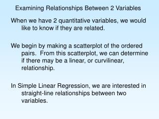
Section 4.1: Fitting a Line by Least Squares • Often we want to fit a straight line to data. • For example from an experiment we might have the following data showing the relationship of density of specimens made from a ceramic compound at different pressures. • By fitting a line to the data we can predict what the average density would be for specimens made at any given pressure, even pressures we did not investigate experimentally.
For a straight line we assume a model which says that on average in the whole population of possible specimens the average density, y, value is related to pressure, x, by the equation • The population (true) intercept and slope are represented by Greek symbols just like m and s.
How to choose the best line?----Principle of least squares • To apply the principle of least squares in the fitting of an equation for y to an n-point data set, values of the equation parameters are chosen to minimize where y1, y2, …, yn are the observed responses and yi-hat are corresponding responses predicted or fitted by the equation.
In another word • We want to choose a slope and intercept so as to minimize the sum of squared vertical distances from the data points to the line in question.
A least squares fit minimizes the sum of squared deviations from the fitted line minimize • Deviations from the fitted line are called “residuals” • We are minimizing the sum of squared residuals, called the “residual sum of squares.”
Come again We need to minimize over all possible values of b0 and b1. This is a calculus problem (take partial derivatives).
The resulting formulas for the least squares estimates of the intercept and slope are • Notice the notation. We use b1 and b0 to denote some particular values for the parameters b1 and b0.
The fitted line • For the measured data we fit a straight line • For the ith point, the fitted value or predicted value is which represent likely y behavior at that x value.
Interpolation • At the situation for x=5000psi, there are no data with this x value. • If interpolation is sensible from a physical view point, the fitted value can be used to represent density for 5,000 psi pressure.
“Least squares” is the optimal method to use for fitting the line if • The relationship is in fact linear. • For a fixed value of x the resulting values of y are • normally distributed with • the same constant variance at all x values.
If these assumptions are not met, then we are not using the best tool for the job. • For any statistical tool, know when that tool is the right one to use.
4.1.2 The Sample Correlation and Coefficient of Determination The sample (linear) correlation coefficient, r, is a measure of how “correlated” the x and y variable are.The correlation is between -1 and 1 +1 means perfect positive linear correlation 0 means no linear correlation -1 means perfect negative linear correlation
The sample correlation is computed by • It is a measure of the strength of an apparent linear relationship.
Coefficient of Determination It is another measure of the quality of a fitted equation.
lnterpretationof R2 R2 = fraction of variation accounted for (explained) by the fitted line.
If we don't use the pressures to predict density • We use to predict every yi • Our sum of squared errors is = SS Total • If we do use the pressures to predict density • We use to predict yi = SS Residual
The percent reduction in our error sum of squares is Using x to predict y decreases the error sum of squares by 98.2%.
The reduction in error sum of squares from using x to predict y is • Sum of squares explained by the regression equation • 284,213.33 = SS Regression This is also the correlation squared. r2 = 0.9912 = 0.982=R2
For a perfectly straight line • All residuals are zero. • The line fits the points exactly. • SS Residual = 0 • SS Regression = SS Total • The regression equation explains all variation • R2 = 100% • r = ±1 r2 = 1 If r=0, then there is no linear relationship between x and y • R2 = 0% • Using x to predict y with a linear model does not help at all.
4.1.3 Computing and Using Residuals • Does our linear model extract the main message of the data? • What is left behind? (hopefully only small fluctuations explainable only as random variation) • Residuals!
Good Residuals: Pattenless • They should look randomly scattered if a fitted equation is telling the whole story. • When there is a pattern, there is something gone unaccounted for in the fitting.
Plotting residuals will be most crucial in section 4.2 with multiple x variables • But residual plots are still of use here. Plot residuals versus • Predicted values • Versus x • In run order • Versus other potentially influential variables, e.g. technician • Normal Plot of residuals Read the book Page 135 for more Residual plots.
Checking Model Adequacy With only single x variable, we can tell most of what we need from a plot with the fitted line.
A residual plot gives us a magnified view of the increasing variance and curvature. This residual plot indicates 2 problems with this linear least squares fit • The relationship is not linear • Indicated by the curvature in the residual plot • The variance is not constant • So the least squares method isn't the best approach even if we handle the nonlinearity.
Some Cautions • Don't fit a linear function to these data directly with least squares. • With increasing variability, not all squared errors should count equally.
Some Study Questions • What does it mean to say that a line fit to data is the "least squares" line? Where do the terms least and squares come from? • We are fitting data with a straight line. What 3 assumptions (conditions) need to be true for a linear least squares fit to be the optimal way of fitting a line to the data? • What does it mean if the correlation between x and y is -1? What is the residual sum of squares in this situation? • If the correlation between x and y is 0, what is the regression sum of squares, SS Regression, in this situation?
What is the value of R2? • What is the least squares regression equation? • How much does y increase on average if x is increased by 1.0? • What is the sum of squared residuals? Do not compute the residuals; find the answer in the Excel output. • What is the sum of squared deviations of y from y bar? • By how much is the sum of squared errors reduced by using x to predict y compared to using only y bar to predict y? • What is the residual for the point with x = 2?