Neural Plasticity and Topographic Organization in Sensory Cortical Areas After Nerve Damage
120 likes | 247 Vues
This study explores the dynamics of neural plasticity in sensory cortical areas, focusing on the topographic maps formed between sensory fields and cortical regions. We examine somatotopic mapping in the somatosensory cortex and retinotopic mapping in the visual cortex, highlighting how these areas reorganize following peripheral nerve damage or digit amputation. Using mathematical models based on neural field theory, we investigate the effects of stimulus amplification and the implications for understanding columnar microstructures in the cerebrum. Our preliminary findings indicate a need for revising existing theories on topographic organization.

Neural Plasticity and Topographic Organization in Sensory Cortical Areas After Nerve Damage
E N D
Presentation Transcript
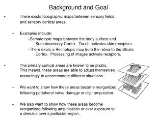
Background and Goal There exists topographic maps between sensory fields and sensory cortical areas. Examples Include: Somatotopic maps between the body surface and Somatosensory Cortex. Touch activates skin receptors. There exists a Retinotopic map from the retina to the Striate Cortex. Processing of images activate receptors. The primary cortical areas are known to be plastic. This means, these areas are able to adjust themselves accordingly to accommodate different situations. We want to show how these areas become reorganized following peripheral nerve damage or digit amputation. We also want to show how these areas become reorganized following amplification or over exposure to a stimulus over a particular region.
Neural Fieldsfrom Dr. Shun-ichi Amari’s Perspective • Mathematical Models of Neural Fields represent Cortical Neural Tissues. • Modified Willshaw-Malsburg Model: represents the mean voltage level at time at cell location represents external stimulus to the Neural Field at at time represents a weight function (Difference of Gaussians also known as the “Mexican Hat” function) since the firing output of a nearby neuron, , will affect other neurons. represents the firing rate of a neuron. A sigmoidal function (blue) is a representation of one such function, but we consider the extreme case whereis a heaviside function (red), where the neuron is either firing at its maximum rate, or not firing at all
Takeuchi-Amari Theory Outside Stimulus A model for the intensity of which neurons at receive the stimulus is given by (Amari 1977): Receptor Field measures the magnitude of presynaptic strength of the neurons at to postsynaptic strength of the nuerons at Neural Field measures the weight of synaptic connections from the inhibitory neuron pool ( ) to neurons at Inhibitory Pool and are regions affecting a subset of and respectively. Here we only investigate only one particular pair at time .
Arriving at The Model The dynamics of and are (Amari 1977): Using the above and A system of 3 Differential Equations is established However, we can derive by differentiating and substituting in the equations of and This will give us the following system of 2 differential equations instead:
Definitions is the probability of a stimulus occurring at This is what we manipulate throughout the investigation represents the rest potential of the nerve cell We define via and as a function which takes the shape of the following plot: indicates we use a small time scale
Previous Work • Takeuchi and Amari, 1979 • Found that topographic organization with columnar microstructures appear when the equilibrium solution of the system is unstable. It is hypothesized this explains the existence of columnar structures in the cerebrum. • Peterson and Taylor, 1996 • Long-term effects on a neural network from behavioral training is observed through a small perturbation analysis off of the uniform state (where ). • Missing (and of interest here) • What happens to the topographic organization should amputation or amplification (large perturbation) occur?
Stationary PatternsTime Independent Let D be the receptor field of active cells defined as: We begin with the case where stimulus is uniformly applied, thus
Test of Neural Field Approach to Sensory Plasticity • How does change for different stimulus conditions (different )? • Strategy: • Determine for uniform case • Modify to represent • Amputation Where = 0 in some sub-region of • Amplification Where is unimodal • Run of the Dynamics to see what becomes
Stationary Solutions2-Region Example Plot of the boundary, Let be some arbitrary monotonically increasing curve. Takeuchi and Amari assumed to be linear. If this was the case, would require conditions on the weight and kernel functions, defined previously, that were found to be unreasonably restrictive and physiologically unreasonable.
Takeuchi-Amari Theoryneeds revision Takeuchi and Amari built their theory on result that ‘s boundary is linear This is incorrect: satisfies a differential equation and has theform: which gives us the following 3D Plot of
Conclusion and Future Directions • Preliminary investigation where we found the underlying previous result of Takeuchi and Amari was not correct. • Basic structure should give insight to neural plasticity when more development is done.
References • Amari, Shun-ichi. “Dynamics of Patter Formation in Lateral-Inhibition Type Neural Fields”. Biological Cybernetics. Vol. 27. 1977: 77-87. • Amari, Shun-ichi and Takeuchi, A. “Formation of Topographic Maps and Columnar Microstructures in Nerve Fields”. Biological Cybernetics. Vol. 35. 1979: 63-72. • Peterson, Rasmus S. and Taylor, John G. “Reorganization of Somatosensory Cortex after Tactile Training”. Advances in Neural Processing Systems. Vol. 2. 1996: 82-88. Acknowledgements This investigation was supported, in part, by the National ScienceFoundation's Research Experiences for Undergraduates Site ProgramDMS-0354034.