Download
1 / 15
150 likes | 249 Vues
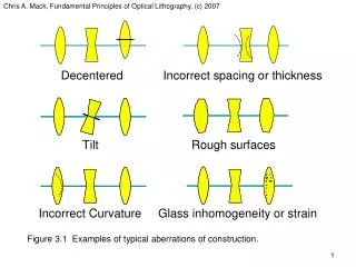
Figure 8.1 When transport occurs along parallel fluxlines, the conservation equation takes the simple form given in equation 8:7. Figure 8.2 When fluxlines are not parallel, the conservation law takes the form given in equation 8:8.

E N D
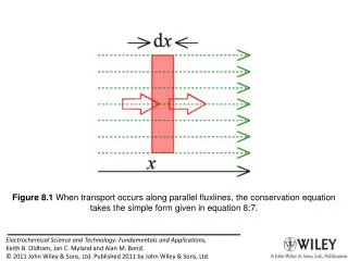
Figure 8.1 When transport occurs along parallel fluxlines, the conservation equation takes the simple form given in equation 8:7.
Figure 8.2 When fluxlines are not parallel, the conservation law takes the form given in equation 8:8.
Figure 8.3 When fluxlines radiate from a point, equiconcentration surfaces are spheres, or portions thereof, and the conservation equation is as reported in 8:9.
Figure 8.4 The Grotthuss mechanism. The exchange of a proton H+ between an ion and a water molecule mimics true migration and inflates the mobility.
Figure 8.5 The motion of the junction between two solutions of known conductivity is measured in the moving boundary method.
Figure 8.7 In the potential-leap experiment, the WE is suddenly brought to a potential large enough to denude the electrode surface of the electroreactant.
Figure 8.8 Concentration profiles resulting from the potential-leap experiment for a diffusivity DR = 1.00 10–9 m2 s–1. Note that, even after times as long830 as 100 s, the concentration diminution is confined to a layer of only about one millimeter thickness, easily validating condition 8:27.
Figure 8.9 A narrow tube interconnects two electrode chambers that are gently stirred to ensure uniform composition in each chamber.
Figure 8.10 Poiseuille flow through a tube. The velocity profile, given byv (r) = 2V [R2–r2]/πR4, where V is the flowrate (m3 s1), is shown in cross section.
Figure 8.11 Geometry of the rotating disk electrode, showing also the flowlines followed by the convecting solution.
Figure 8.12 Coordinates useful in describing the behavior of the solution adjacent to a rotating disk electrode.
Figure 8.13 The concentration profile at a rotating disk electrode according to equation 8:48. The graph is correctly scaled for the typical value b = (18 μm)3.
Figure 8.14 Concentration profiles during the experiment analyzed in Web#852. The neutral species R and the cation O are involved in the electrode reaction R(soln) ⇄ e– + O(soln), while C and A are the cation and anion of the supporting electrolyte.
Figure 8.15 Flux density profiles corresponding to the concentrations shown inFigure 8-14. Notice the transition from the transport being largely that of the electroactive species close to the electrode to being predominantly that of the supporting ions in the bulk. See Web#852 for details.