Regression Modeling for Predicting Drug Cost and Gas Mileage
Learn how to estimate parameters in polynomial and multiple regression models for predicting drug production costs and gas mileage. Explore examples and equations to understand the process.

Regression Modeling for Predicting Drug Cost and Gas Mileage
E N D
Presentation Transcript
Polynomial RegressionFor k th-degree model:Y=0 + 1x + 2x2 +…+ kxk + Where is N(0, 2)
Least Squares Equations For Estimation of Polynomial-Regression ParametersFor k + 1 equations:0n + 1x+ 2x2+…+ kxk = y0x+ 1x2+ 2x3+…+ kxk+1 = xy : : : : : : : : : :0xk+ 1xk+1+ ………+ kx2k = xky
Example: Least Squares Polynomial Regression ModelA study is conducted to develop an equation by which the unit cost of producing a new drug (Y) can be predicted based on the number on units produced (X). Data collected for the study follows:Number (units) Cost Number (units) Cost (x$100) 5 14.0 15 1.8 5 12.5 20 6.2 10 7.0 20 4.9 10 5.0 25 13.2 15 2.1 25 14.6 A XY-scatter chart of these data suggest a quadratic model. Find the parameters of this model using the Least Squares principle.
Estimator for 2 S2 = SSEn – (k+1)SSE = [y2 – (y)2/n] – [0y + 1x1y + 2x2y+…+ kxky – (y)2/n]General equation for Polynomial & Multiple Regression estimation of Random Error 2.
Coefficient of Multiple Determinationr2 = SSR SYYSSR = [0y + 1x1y +2x2y+…+ kxky – (y)2/n]SYY = [y2 – (y)2/n] SSR is the Regression Sum of Squares.SYY is the Corrected Total Sum of Squares.
Multiple RegressionFor k th-degree model:Y=0 + 1x1 + 2x2 +…+ kxk + Where is N(0, 2)For independent variables x1, x2, …, x3
Least Squares Equations For Estimation of Multiple-Regression ParametersFor k + 1 equations:0n + 1x1 + 2x2 +…+ kxk = y0x1 + 1x21 + 2x1x2+…+ kx1xk = x1y : : : : : : : : : :0xk + 1xkx1 + 2xkx2 +…+ kx2k = xkyIt is possible to construct other models by forming variables that are mathematical functions of x1 and/or x2.
Example: Multiple RegressionA project is designed to develop an equation which will be able to predict the gasoline mileage of an automobile based on its weight and the temperature at the time of operation. These data are collected: Car 1 2 3 4 5 6 7 8 9 10 mpg |17.9 16.5 16.4 16.8 18.8 15.5 17.5 16.4 15.9 18.3 tons |1.35 1.90 1.70 1.80 1.30 2.05 1.60 1.80 1.85 1.40 oF | 90 30 80 40 35 45 50 60 65 30x1 = 16.75 x2 = 525 x1x2 = 874.5x12 = 28.6375 x22 = 31,475 x1y = 282.405y = 170 x2y = 8,887 y2 = 2,900.46 The project also requires an estimate of 2 and what proportion of the total variability in Y can be explained by our fitted regression model.
Example: Multiple RegressionA project is designed to measure the pull strength of a wire bond in a semiconductor manufacturing process. The finished semiconductor is wire bonded to a frame. The independent variables of interest are wire length (x1) and die height (x2). Use the method of least squares to estimate the regression coefficients in a multiple regression model utilizing both variables to predict pull strength of wire bonds. Summary data for (25) observations follow:x1 = 206 x2 = 8,294 x1x2 = 77,177 x12 = 2,396 x22 = 3,531,848 x1y = 8,008.37y = 725.82 x2y = 274,811.31 y2 = 27,177.951 Also estimate the true random error (2) for the multiple regression model and provide a measure of the adequacy.
Multiple Regression ExampleThe data listed below represent the percent of impurities that occurred at various temperatures and sterilizing times during a reaction associated with the manufacturing of an alcoholic beverage. Estimate the regression coefficients using the method of least squares. Fit a complete second-order or full quadratic model with interaction to the data.Sterilizing Temperature, x1 (OC)Time, x2 (min) 75 100 125 15 >>> 14.05 10.55 7.55 14.93 9.48 6.5920>>> 16.56 13.63 9.23 15.85 11.75 8.7825>>> 22.41 18.55 15.93 21.66 17.98 16.44See Spread Sheet For Summations
Nonlinear Exponential Modely = ex Transformed Linear Model:y’ = 0’ + 1‘x + ’Where: > y’ = ln(y) > 0’ = ln() > 1’= > ’ = ln()
Nonlinear Least Squares Estimates of Parameters1’ = SXY = x’y’– [(x’)(y’) / n] SXX(x’2) – [(x’)2 / n]0’ = y’ - 1x’s2= SSE = (y’)2 - 0’y’- 1’x’y’ n – 2 n – 2
Example: Exponential ModelAstronomers discover new quasars by surveying the sky for star-like objects whose colors differ from ordinary stars. A study on radio galaxies (type 1 quasars) found that for class S galaxies, Luminosity (y) in MHz is exponentially related to its visible-light Spectra (absorption lines) Index (x).Representative data appears here:Spectra Index: .59 .67 .72 .80 .85 .90 ln (L): 23.6 25.6 26.4 25.7 26.8 26.7Spectra Index: .94 .66 1.00 .86 1.03 .70 ln (L): 27.0 24.9 27.1 27.2 26.9 25.2Estimate the parameters of the exponential model.What value of L would you predict for a spectral index of .75?
Nonlinear Power Modely = 0 x1 Transformed Linear Model:y’ = 0’ + 1’x’ + ’Where: > y’ = log (y) or ln (y) > 0’ = log (0) or ln (0) > 1’= 1 or 1 > x’ = log (x) or ln (x) > ’ = log() or ln ()
Nonlinear Power Model Example Feature recognition from surface models of complicated parts is becoming increasingly important in the development of efficient CAD systems. An experiment tracks recognition time (y) to the number of edges (x) of a given part. A graph of log10 (total recognition time in seconds) versus log10 (number of edges) is plotted. Does a scatter plot of log values suggest an approximate linear relationship between these two variables? What probabilistic model is implied by the simple linear regression relationship between the transformed variables? Calculate estimates of the parameters & predict the time when the number of edges is equal to 300. (See log-values “plot” on next page). Log data: Log (edges): 1.1 1.5 1.7 1.9 2.0 2.1 2.2 2.3 2.7 Log (time): .30 .50 .55 .52 .85 .98 1.10 1.00 1.18 Log(edges): 2.8 3.0 3.3 3.5 3.8 4.2 4.3 Log (time): 1.45 1.65 1.84 2.05 2.46 2.50 2.76 n= 16 Σx΄ = 42.4 Σy΄= 21.69 Σx΄2 = 126.34 Σy΄2 = 38.5305 Σx΄y΄ = 68.64
Nonlinear Reciprocal Modely = 0 + 1 (1/x) + Transformed Linear Model:y = 0 + 1x’ + Where: x’ = 1/x
Example of Nonlinear Reciprocal Sample data suggests that the expected value of the thermal conductivity of polyethylene (y) is a linear function of 104 * 1/x where (x) is lamellar thickness. Estimate parameters of the regression function. Predict the value of thermal conductivity when lamellar thickness is 500 A (1A = 10-10m). Data: X| 240 410 460 490 520 590 745 8,300 y|12.0 14.7 14.7 15.2 15.2 15.6 16.0 18.1 Σx΄= 159.01; Σy = 121.5; Σx΄2 = 4,058.8 Σy2 = 1,865.2; Σx΄y = 2,281.6