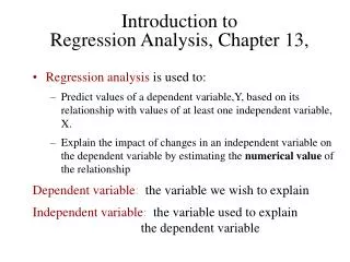
Chapter 13 Introduction to Multiple Regression
Statistics for Managers Using Microsoft ® Excel 4 th Edition Chapter 13 Introduction to Multiple Regression The Multiple Regression Model Idea: Examine the linear relationship between 1 dependent (Y) & 2 or more independent variables (X i )

Chapter 13 Introduction to Multiple Regression
E N D
Presentation Transcript
Statistics for Managers Using Microsoft® Excel4th Edition Chapter 13 Introduction to Multiple Regression Statistics for Managers Using Microsoft Excel, 4e © 2004 Prentice-Hall, Inc.
The Multiple Regression Model Idea: Examine the linear relationship between 1 dependent (Y) & 2 or more independent variables (Xi) Multiple Regression Model with k Independent Variables: Population slopes Random Error Y-intercept Statistics for Managers Using Microsoft Excel, 4e © 2004 Prentice-Hall, Inc.
Multiple Regression Equation The coefficients of the multiple regression model are estimated using sample data Multiple regression equation with k independent variables: Estimated (or predicted) value of Y Estimated intercept Estimated slope coefficients In this chapter we will always use Excel to obtain the regression slope coefficients and other regression summary measures. Statistics for Managers Using Microsoft Excel, 4e © 2004 Prentice-Hall, Inc.
Multiple Regression Equation (continued) Two variable model Y Slope for variable X1 X2 Slope for variable X2 X1 Statistics for Managers Using Microsoft Excel, 4e © 2004 Prentice-Hall, Inc.
Example: 2 Independent Variables • A distributor of frozen desert pies wants to evaluate factors thought to influence demand • Dependent variable: Pie sales (units per week) • Independent variables: Price (in $) Advertising ($100’s) • Data are collected for 15 weeks Statistics for Managers Using Microsoft Excel, 4e © 2004 Prentice-Hall, Inc.
Pie Sales Example Multiple regression equation: Sales = b0 + b1 (Price) + b2 (Advertising) Statistics for Managers Using Microsoft Excel, 4e © 2004 Prentice-Hall, Inc.
Estimating a Multiple Linear Regression Equation • Excel will be used to generate the coefficients and measures of goodness of fit for multiple regression • Excel: • Tools / Data Analysis... / Regression Statistics for Managers Using Microsoft Excel, 4e © 2004 Prentice-Hall, Inc.
Multiple Regression Output Statistics for Managers Using Microsoft Excel, 4e © 2004 Prentice-Hall, Inc.
The Multiple Regression Equation where Sales is in number of pies per week Price is in $ Advertising is in $100’s. b1 = -24.975: sales will decrease, on average, by 24.975 pies per week for each $1 increase in selling price, net of the effects of changes due to advertising b2 = 74.131: sales will increase, on average, by 74.131 pies per week for each $100 increase in advertising, net of the effects of changes due to price Statistics for Managers Using Microsoft Excel, 4e © 2004 Prentice-Hall, Inc.
Using The Equation to Make Predictions Predict sales for a week in which the selling price is $5.50 and advertising is $350: Note that Advertising is in $100’s, so $350 means that X2 = 3.5 Predicted sales is 428.62 pies Statistics for Managers Using Microsoft Excel, 4e © 2004 Prentice-Hall, Inc.
Coefficient of Multiple Determination • Reports the proportion of total variation in Y explained by all X variables taken together Statistics for Managers Using Microsoft Excel, 4e © 2004 Prentice-Hall, Inc.
Multiple Coefficient of Determination (continued) 52.1% of the variation in pie sales is explained by the variation in price and advertising Statistics for Managers Using Microsoft Excel, 4e © 2004 Prentice-Hall, Inc.
Adjusted r2 • r2 never decreases when a new X variable is added to the model • This can be a disadvantage when comparing models • What is the net effect of adding a new variable? • We lose a degree of freedom when a new X variable is added • Did the new X variable add enough explanatory power to offset the loss of one degree of freedom? Statistics for Managers Using Microsoft Excel, 4e © 2004 Prentice-Hall, Inc.
Adjusted r2 (continued) • Shows the proportion of variation in Y explained by all X variables adjusted for the number of Xvariables used (where n = sample size, k = number of independent variables) • Penalize excessive use of unimportant independent variables • Smaller than r2 • Useful in comparing among models Statistics for Managers Using Microsoft Excel, 4e © 2004 Prentice-Hall, Inc.
Adjusted r2 (continued) 44.2% of the variation in pie sales is explained by the variation in price and advertising, taking into account the sample size and number of independent variables Statistics for Managers Using Microsoft Excel, 4e © 2004 Prentice-Hall, Inc.
Simple and Multiple Regression Compared • Coefficients in a simple regression pick up the impact of that variable plus the impacts of other variables that are correlated with it and the dependent variable. • Coefficients in a multiple regression net out the impacts of other variables in the equation. Statistics for Managers Using Microsoft Excel, 4e © 2004 Prentice-Hall, Inc.
Simple and Multiple Regression Compared:Example • Two simple regressions: • ABSENCES=a+b1AUTONOMY • ABSENCES= a +b2SKILLVARIETY • Multiple Regression: • ABSENCES= a +b1AUTONOMY+ b2SKILLVARIETY Statistics for Managers Using Microsoft Excel, 4e © 2004 Prentice-Hall, Inc.
Venn Diagrams and Regression Statistics for Managers Using Microsoft Excel, 4e © 2004 Prentice-Hall, Inc.
Venn Diagrams and Regression Statistics for Managers Using Microsoft Excel, 4e © 2004 Prentice-Hall, Inc.
Overlap in Explanation Statistics for Managers Using Microsoft Excel, 4e © 2004 Prentice-Hall, Inc.
Is the Model Significant? • F-Test for Overall Significance of the Model • Shows if there is a linear relationship between all of the X variables considered together and Y • Use F test statistic • Hypotheses: H0: β1 = β2 = … = βk = 0 (no linear relationship) H1: at least one βi≠ 0 (at least one independent variable affects Y) Statistics for Managers Using Microsoft Excel, 4e © 2004 Prentice-Hall, Inc.
F-Test for Overall Significance • Test statistic: where F has (numerator) = k and (denominator) = (n – k - 1) degrees of freedom Statistics for Managers Using Microsoft Excel, 4e © 2004 Prentice-Hall, Inc.
F-Test for Overall Significance (continued) With 2 and 12 degrees of freedom P-value for the F-Test Statistics for Managers Using Microsoft Excel, 4e © 2004 Prentice-Hall, Inc.
H0: β1 = β2 = 0 H1: β1 and β2 not both zero = .05 df1= 2 df2 = 12 F-Test for Overall Significance (continued) Test Statistic: Decision: Conclusion: Critical Value: F = 3.885 Since F test statistic is in the rejection region (p-value < .05), reject H0 = .05 0 F There is evidence that at least one independent variable affects Y Do not reject H0 Reject H0 F.05 = 3.885 Statistics for Managers Using Microsoft Excel, 4e © 2004 Prentice-Hall, Inc.
Are Individual Variables Significant? • Use t-tests of individual variable slopes • Shows if there is a linear relationship between the variable Xi and Y • Hypotheses: • H0: βi = 0 (no linear relationship) • H1: βi≠ 0 (linear relationship does exist between Xi and Y) Statistics for Managers Using Microsoft Excel, 4e © 2004 Prentice-Hall, Inc.
Are Individual Variables Significant? (continued) H0: βi = 0 (no linear relationship) H1: βi≠ 0 (linear relationship does exist between xi and y) Test Statistic: (df = n – k – 1) Statistics for Managers Using Microsoft Excel, 4e © 2004 Prentice-Hall, Inc.
Are Individual Variables Significant? (continued) t-value for Price is t = -2.306, with p-value .0398 t-value for Advertising is t = 2.855, with p-value .0145 Statistics for Managers Using Microsoft Excel, 4e © 2004 Prentice-Hall, Inc.
H0: βi = 0 H1: βi 0 Inferences about the Slope: tTest Example From Excel output: • d.f. = 15-2-1 = 12 • = .05 t/2 = 2.1788 The test statistic for each variable falls in the rejection region (p-values < .05) Decision: Conclusion: Reject H0 for each variable a/2=.025 a/2=.025 There is evidence that both Price and Advertising affect pie sales at = .05 Reject H0 Do not reject H0 Reject H0 -tα/2 tα/2 0 -2.1788 2.1788 Statistics for Managers Using Microsoft Excel, 4e © 2004 Prentice-Hall, Inc.
Job Earnings Example • http://www.ilir.uiuc.edu/courses/lir593/jearnoutput.htm • ERTEN: 27.4/2.5= 10.9 t1171 • UNEM: -229.1/45.9= -5.0 t1171 • EDU: 885.13/76.5= 11.6 t1171 Statistics for Managers Using Microsoft Excel, 4e © 2004 Prentice-Hall, Inc.
Confidence Interval Estimate for the Slope Confidence interval for the population slope βi where t has (n – k – 1) d.f. Here, t has (15 – 2 – 1) = 12 d.f. Example: Form a 95% confidence interval for the effect of changes in price (X1) on pie sales: -24.975 ± (2.1788)(10.832) So the interval is (-48.576 , -1.374) Statistics for Managers Using Microsoft Excel, 4e © 2004 Prentice-Hall, Inc.
Confidence Interval Estimate for the Slope (continued) Confidence interval for the population slope βi Example: Excel output also reports these interval endpoints: Weekly sales are estimated to be reduced by between 1.37 to 48.58 pies for each increase of $1 in the selling price Statistics for Managers Using Microsoft Excel, 4e © 2004 Prentice-Hall, Inc.
Qualitative Independent Variables • Can we handle variable such as gender or race or state or schooling categories in a regression? • YES. In fact, we can exactly duplicate ANOVA (differences of means across categories) and t-tests for differences of means with regression. • Therefore, regression can handle almost all the tests that we have previously done! Statistics for Managers Using Microsoft Excel, 4e © 2004 Prentice-Hall, Inc.
Using Dummy Variables • A dummy variable is a categorical explanatory variable with two levels: • yes or no, on or off, male or female • coded as 0 or 1 • Regression intercepts are different if the variable is significant • If more than two levels, the number of dummy variables needed is (number of levels - 1) Statistics for Managers Using Microsoft Excel, 4e © 2004 Prentice-Hall, Inc.
Regression with only dummy variables • Two sample t-test: Suppose that we have two groups: M and F and we want to know if their job satisfaction is the same. • Code variable female=1 if the person is female and female=0 if male • JS = α + β1FEMALE • Then for males the equation predicts: • JS = α + β1(0) = α therefore α is the avg of JS for males • For females the equation predicts: • JS = α + β1(1) = α + β1 therefore α + β1 is avg of JS for females Statistics for Managers Using Microsoft Excel, 4e © 2004 Prentice-Hall, Inc.
Regression with only dummy variables • Thus, β1 is the difference of means in JS for males and females. The t-test is identical to the test that we did previously! • Now suppose that we have 3 groups: Blacks, Whites and Asians. We form TWO dummies variables (# groups – 1). For example, BLACK=1 iff race is Black and ASIAN=1 iff race is Asian and zero otherwise Statistics for Managers Using Microsoft Excel, 4e © 2004 Prentice-Hall, Inc.
Regression with only dummy variables • The regression is JS= α + β1ASIAN + β2BLACK • For Whites JS= α + β1(0) + β2(0) = α • For Blacks JS= α + β1(0) + β2(1) = α + β2 • For Asians JS= α + β1(1) + β2(0) = α + β1 • Therefore, the coefficients on ASIAN and BLACK represent the difference of means of that group and the EXCLUDED group (Whites) • What is the difference of means between Asians and Blacks? Statistics for Managers Using Microsoft Excel, 4e © 2004 Prentice-Hall, Inc.
Regression with only dummy variables • To test the hypothesis that there is a difference of means across the 3 groups, we can just use the F-test for the entire regression. • This yields an IDENTICAL test to One-way ANOVA! • These tests can be generalized to include continuous variables and interactions Statistics for Managers Using Microsoft Excel, 4e © 2004 Prentice-Hall, Inc.
Dummy-Variable Example (with 2 Levels) and 1 continuous variable Let: Y = pie sales X1 = price X2 = holiday (X2 = 1 if a holiday occurred during the week) (X2 = 0 if there was no holiday that week) Statistics for Managers Using Microsoft Excel, 4e © 2004 Prentice-Hall, Inc.
Dummy-Variable Example (with 2 Levels) (continued) Holiday No Holiday Different intercept Same slope Y (sales) If H0: β2 = 0 is rejected, then “Holiday” has a significant effect on pie sales b0 + b2 Holiday (X2 = 1) b0 No Holiday (X2 = 0) X1 (Price) Statistics for Managers Using Microsoft Excel, 4e © 2004 Prentice-Hall, Inc.
Interpreting the Dummy Variable Coefficient (with 2 Levels) Example: Sales: number of pies sold per week Price: pie price in $ Holiday: 1 If a holiday occurred during the week 0 If no holiday occurred b2 = 15: on average, sales were 15 pies greater in weeks with a holiday than in weeks without a holiday, given the same price Statistics for Managers Using Microsoft Excel, 4e © 2004 Prentice-Hall, Inc.
Dummy-Variable Models (more than 2 Levels) • The number of dummy variables is one less than the number of levels • Example: Y = house price ; X1 = square feet • If style of the house is also thought to matter: Style = ranch, split level, condo Three levels, so two dummy variables are needed Statistics for Managers Using Microsoft Excel, 4e © 2004 Prentice-Hall, Inc.
Dummy-Variable Models (more than 2 Levels) (continued) • Example: Let “condo” be the default category, and let X2 and X3 be used for the other two categories: Y = house price X1 = square feet X2 = 1 if ranch, 0 otherwise X3 = 1 if split level, 0 otherwise The multiple regression equation is: Statistics for Managers Using Microsoft Excel, 4e © 2004 Prentice-Hall, Inc.
Interpreting the Dummy Variable Coefficients (with 3 Levels) Consider the regression equation: For a condo: X2 = X3 = 0 With the same square feet, a ranch will have an estimated average price of 23.53 thousand dollars more than a condo For a ranch: X2 = 1; X3 = 0 With the same square feet, a split-level will have an estimated average price of 18.84 thousand dollars more than a condo. For a split level: X2 = 0; X3 = 1 Statistics for Managers Using Microsoft Excel, 4e © 2004 Prentice-Hall, Inc.
Testing Portions of the Multiple Regression Model • Contribution of a Single Independent Variable Xj SSR(Xj | all variables except Xj) = SSR (all variables) – SSR(all variables except Xj) • Measures the contribution of Xj in explaining the total variation in Y (SST) Statistics for Managers Using Microsoft Excel, 4e © 2004 Prentice-Hall, Inc.
Testing Portions of the Multiple Regression Model (continued) • Contribution of a Single Independent Variable Xj, assuming all other variables are already included • (consider here a 3-variable model): • SSR(X1 | X2 and X3) • = SSR (all variables) – SSR(X2 and X3) From ANOVA section of regression for From ANOVA section of regression for Measures the contribution of X1 in explaining SST Statistics for Managers Using Microsoft Excel, 4e © 2004 Prentice-Hall, Inc.
The Partial F-Test Statistic • Consider the hypothesis test: H0: variable Xj does not significantly improve the model after all other variables are included H1: variable Xj significantly improves the model after all other variables are included • Test using the F-test statistic: (with 1 and n-k-1 d.f.) Statistics for Managers Using Microsoft Excel, 4e © 2004 Prentice-Hall, Inc.
Testing Portions of Model: Example Example: Frozen desert pies Test at the = .05 level to determine whether the price variable significantly improves the model given that advertising is included Statistics for Managers Using Microsoft Excel, 4e © 2004 Prentice-Hall, Inc.
Testing Portions of Model: Example (continued) H0: X1 (price) does not improve the model with X2 (advertising) included H1: X1 does improve model = .05, df = 1 and 12 F critical Value = 4.75 (For X1 and X2) (For X2 only) Statistics for Managers Using Microsoft Excel, 4e © 2004 Prentice-Hall, Inc.
Testing Portions of Model: Example (continued) (For X1 and X2) (For X2 only) Conclusion: Reject H0; adding X1 does improve model Statistics for Managers Using Microsoft Excel, 4e © 2004 Prentice-Hall, Inc.
Do I need to do this for one variable? • The F test for the inclusion of a single variable after all other variables are included in the model isIDENTICAL to the t test of the slope for that variable • The only reason to do an F test is to test several variables together. Statistics for Managers Using Microsoft Excel, 4e © 2004 Prentice-Hall, Inc.