More solution methods for the TSP
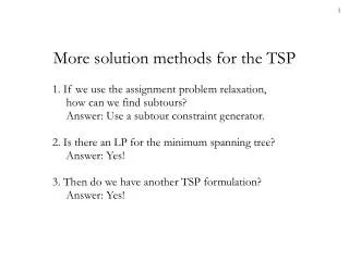
More solution methods for the TSP. 1. If we use the assignment problem relaxation, how can we find subtours? Answer: Use a subtour constraint generator. 2. Is there an LP for the minimum spanning tree? Answer: Yes! 3. Then do we have another TSP formulation? Answer: Yes!.

More solution methods for the TSP
E N D
Presentation Transcript
More solution methods for the TSP 1. If we use the assignment problem relaxation,how can we find subtours?Answer: Use a subtour constraint generator. 2. Is there an LP for the minimum spanning tree?Answer: Yes! 3. Then do we have another TSP formulation?Answer: Yes!
We’ll use this example today (Winston). • Looks like subtours are likely!
Solve the assignment problem relaxation • min 1.4 x1,2 + 3.6 x1,3 + 6.4 x1,4 + 7 x1,5 + 7.6 x1,6+ 2.2 x2,3 + 6.7 x2,4 + 6.1 x2,5 + 7.2 x2,6 + 8.2 x3,4+ 5.8 x3,5 + 7.8 x3,6 + 5.8 x4,5 + 3.6 x4,6 + 3 x5,6, • Degrees1: x1,2 + x1,3 + x1,4 + x1,5 + x1,6 = 2, • Degrees2: x1,2 + x2,3 + x2,4 + x2,5 + x2,6 = 2, • Degrees3: x1,3 + x2,3 + x3,4 + x3,5 + x3,6 = 2, • Degrees4: x1,4 + x2,4 + x3,4 + x4,5 + x4,6 = 2, • Degrees5: x1,5 + x2,5 + x3,5 + x4,5 + x5,6 = 2, • Degrees6: x1,6 + x2,6 + x3,6 + x4,6 + x5,6 = 2. • Solution arcs: (1,2), (1,3), (2,3), (4,5), (4,6), (5,6). • Where are the subtours?We could find them by inspection,but we need something we can program.
Let’s write a math model to find subtours! • The problem with subtours is that our salesmancan flow in & out of each city, but not from city 1 to each city. • If the subtours were pipes, and we tried to flow from node 1 to node 5, we would have flow of zero. • This shows the subtour! • Let’s use a max flow model, from node 1 to each node i. • If flow from node 1 to i is zero, then we have a subtour.
Formulation for the max flow problem • Indices: i, j, k = nodes. Source node is s. Terminal node is t. • Parameters: cij= pipe capacity between node i and node j. • Dec. variables:zij= flow between nodesi and j. • Model: 1) maximise i zsi • 2) i zij – k zjk = 0 for each node j, • 3) j zsj = i zit, • 4) zij cij, • 5) zij 0. • Explanation: 1) Maximise total flow. • 2) Flow in = flow out for each node. • 3) Flow out of the source s = flow into the terminal t. • 4) Flow on each pipe is less than capacity. • 5) Flows cannot be negative. • As easy to solve as the shortest path problem. They’re dual to each other.
How do we find subtours with a max flow model? • Underscore xij to show it’s fixed. It’s a parameter in the max flow model. • In the max flow model, set link capacity to be the TSP solution, xij. • Indices: i, j, k = nodes. Source node is 1. Terminal node is t. • Parameters: xij= pipe capacity between node i and node j. • Dec. variables:zij= flow between nodesi and j. • For each node t = 2,…, n, maximise the flow from 1 to t: • 1. maximise i z1i • 2. i zij – k zjk = 0 for each node j, • 3. j z1j = i zit, • 4. – xij zij xij, • We allow back flows in the symmetric TSP, so zij could be < 0 (row 4). • The source is node 1. Solve the model n – 1 times, one for each node t.
Example: arcs (1,2), (1,3), (2,3), (4,5), (4,6), (5,6). • maximize flow from node 1 to node 2:max z1,2 + z1,3, • Conserveflow3: z1,3 + z2,3 = 0, • Conserveflow4: – z4,5 – z4,6 = 0, • Conserveflow5: z4,5 – z5,6 = 0, • Conserveflow6: z4,6 + z5,6 = 0. • For xij = 0, we require zij = 0. For xij > 0, we allow –1 ≤ zij ≤ 1. • Solution z1,2 = 1, z1,3 = 1, z2,3 = –1, z4,5= –1, z4,6 = 1, z5,6= –1. • Some are negative! Just flow in the opposite direction, from 6 to 5. • Objective value 2, which means that node 2 has degree 2.No surprise, since the traveler can go from node 1 to node 2.Note that there is no way to flow from 1,2,3 to 4,5,6.
Same thing will happen for node 3. • Same objective.Add the row for 2, drop the row for 3. • maximize flow from node 1 to node 3:max z1,2 + z1,3, • Conserveflow2: z1,2 - z2,3 = 0, • Conserveflow4: - z4,5 - z4,6 = 0, • Conserveflow5: z4,5 - z5,6 = 0, • Conserveflow6: z4,6 + z5,6 = 0. • For xij = 0, we require zij = 0. For xij > 0, we allow –1 ≤ zij ≤ 1. • Similar soln, z1,2 = 1, z1,3 = 1, z2,3=1, z4,5= –1, z4,6 = 1, z5,6= –1. • Objective value 2, which means that node 3 has degree 2.No surprise, since the traveler can go from node 1 to node 3. • But what will happen with node 4?
What about node 4? • maximize flow from node 1 to node 4:max z1,2 + z1,3, • dual price • Conserveflow2: z1,2 - z2,3 = 0, 1, • Conserveflow3: z1,3 + z2,3 = 0, 1, • Conserveflow5: z4,5 – z5,6 = 0, 0, • Conserveflow6: z4,6 + z5,6 = 0, 0. • For xij = 0, we require zij = 0. For xij > 0, we allow –1 ≤ zij ≤ 1. • Solution : z1,2 = –1, z1,3 = 1, z2,3=–1, z4,5 = –1, z4,6 = 1, z5,6 = –1. • Optimal value: Zero flow! So nodes 1 and 4 are in different subtours. • The dual prices tell us what to do.We could increase flow from node 1 to 4, with more capacity at 2 & 3.So create a subtour-breaking constraint with nodes 1, 2 and 3:x1,2 + x1,3 + x2,3 ≤ 2.
The subtour constraint generator. • We start with no subtours, then find subtours, and add them to set R. • Step 0. Set R = empty. • Step 1. Solve the TSP only for subtours in set R. Get solution xij.1. min ij>i cij xij,2. j<i xji+ j>i xij = 2 for all i,3. i,jS xij |S| – 1, for each subset S in R,4. xij {0, 1} for all i, j. • Step 2. For each node t = 2, …, n, solve a max flow to find subtours:5. Maximise Flowt = maximise i z1i,6. i zij – k zjk = 0 for each node j, (dual price λj)7. j z1j = i zit,8. – xij zij xij. • Step 3. If Flowt < 2, then for λj > 0, add node j to a subtour set in R.Go back to Step 1. AMPL code attached.
Typical solution process in AMPL • ampl: commands tsp2.run; Get started. • CPLEX 8.1.0: optimal solution; objective 19.6 First solution to TSP. • CPLEX 8.1.0: optimal solution; objective 2 Max flow – no subtour. • CPLEX 8.1.0: optimal solution; objective 2 Max flow – no subtour. • CPLEX 8.1.0: optimal solution; objective 0 Max flow – subtour! • CPLEX 8.1.0: optimal solution; objective 22.4 Second solution to TSP. • CPLEX 8.1.0: optimal solution; objective 2 Max flow – no subtour. • CPLEX 8.1.0: optimal solution; objective 2 Max flow – no subtour. • CPLEX 8.1.0: optimal solution; objective 2 Max flow – no subtour. • CPLEX 8.1.0: optimal solution; objective 2 Max flow – no subtour. • CPLEX 8.1.0: optimal solution; objective 2 Max flow – no subtour. • ampl: Done!
Comments on the subtour generator • The subtour generator algorithm is usedin the best known TSP algorithms. • A typical algorithm does the following:(1) use a heuristic to find a good upper bound,(2) use the Held-Karp relaxation to get a good lower bound,(3) then run the subtour generator algorithm to find optimality. • This works because finding subtours with the max flow problem is easy.Simplex is not needed for the max flow problem. • Question: If finding subtours is easy,and “no subtours” is the same as a tree or 1-tree,why can’t we use simplex for the min spanning tree?Answer: we can!
Converting max flow to MST • Let’s look at the max flow problem.We solved it for each node t.We could subscript the zij with the node t. • Indices: i, j, k = nodes. Source node is 1. Terminal node is t. • Parameters: xij= pipe capacity between node i and node j. • Dec. variables:ztij= flow between nodesi and j in problem t. • Max flow from 1 to t: 1. maximise i zt,i,t 2. i zt,i,j – k zt,j,k = 0 for all j, t, 3. j zt,1,j = i zt,i,t, for each node t, 4. – xi,j zt,i,j xi,j, for all i, j, t. • The variables mean the flow from each node across an arc. • R. Kipp Martin showed how to convert this to an MST formulation.
An LP formulation for the min spanning tree • Indices: i, j, k = nodes. • Variables:xij = 1 if arc i, j is in the tree, else 0. • zt,i,j= flow from node t to node i through j. • 1. Minimise tree length: min ij>i cij xij, • 2. Capacity from t to i: Σj:j>izt,i,j + Σj:j<izt,i,j ≤ 1, for all t, i, • 3. Upper bounds: zt,i,j ≤ 1, all t, i, j, and zi,i,j = 0, • 4. Capacity from i to j: xi,j = zt,i,j + zt,j,i, for all t, i, j, • 5. Use n – 1 arcs: ijxij = n – 1. • 6. Nonnegativity: xi,j, zt,i,j ≥ 0. • This formulation is naturally integer.We can easily modify it to be a formulation for the TSP.Unfortunately, the n3 variables is probably unrealistic. • Ref: Martin, R. Kipp, “Using Separation Algorithms to Generate MixedInteger Model Reformulations,” Operations Res. Letters, 10 (1991) 119-128. Kipp Martin
Parts of the MST model.It’s huge, n3 variables,but naturally integer. • min 1.4 x0,1 + 3.6 x0,2 + 6.4 x0,3 + … + 3.6 x3,5 + 3 x4,5, • x0,1 + x0,2 + x0,3 + … + x3,4 + x3,5 + x4,5 = 5, • x0,1 - z0,1,0 = 0, • x0,2 - z0,2,0 = 0, • …, • x1,2 - z0,1,2 - z0,2,1 = 0, • x1,3 - z0,1,3 - z0,3,1 = 0, • …, • x0,1 - z1,0,1 = 0, • x0,2 - z1,0,2 - z1,2,0 = 0, • …, • x0,1 - z5,0,1 - z5,1,0 = 0, • x0,2 - z5,0,2 - z5,2,0 = 0, • …, • x3,5 - z5,3,5 = 0, • x4,5 - z5,4,5 = 0, • z0,1,0 + z0,1,2 + z0,1,3 + z0,1,4 + z0,1,5 ≤ 1, • z0,2,0 + z0,2,1 + z0,2,3 + z0,2,4 + z0,2,5 ≤ 1, • z0,3,0 + z0,3,1 + z0,3,2 + z0,3,4 + z0,3,5 ≤ 1, • …, • z3,4,0 + z3,4,1 + z3,4,2 + z3,4,3 + z3,4,5 ≤ 1, • z3,5,0 + z3,5,1 + z3,5,2 + z3,5,3 + z3,5,4 ≤ 1, • z4,5,0 + z4,5,1 + z4,5,2 + z4,5,3 + z4,5,4 ≤ 1. Solution arcs: (1, 2), (2, 3), (3, 5), (4, 6), (5, 6).
Converting Martin’s MST model to a TSP • Just copy node 1 to node n+1, and add degree = 2 constraints. • This is as tight as the DFJ formulation with all subtour breaking rows! • 1. Minimise tree length: min ij>i cij xij, • 2. Capacity from t to i: Σj:j>izt,i,j + Σj:j<izt,i,j ≤ 1, for all t, i. • 3. Upper bounds: zt,i,j ≤ 1, all t, i, j, and zi,i,j = 0. • 4. Capacity from i to j: xi,j = zt,i,j + zt,j,i, for all t, i, j, • 5. Use n arcs: ijxij = n, • 6. Degree 2, except 1 & n+1: j<i xji+ j>i xij = 2 for all i1, i n+1. • 7. Nonnegativity: xi,j, zt,i,j {0,1}. Not naturally integer! • Solution possibilities? • Relax row 6 & solve with column generation. Subproblem is the MST.When done with column generation, solve the master as IP.We have a good upper bound & a good lower bound!
Another hint for the TSP homework • We want to solve min cx, Ax≥ b, x{0,1}, but it has too many variables. • Suppose we have a feasible solution, x. Then cx is an upper bound. • Suppose we solve min cx, Ax ≥ b, x ≥ 0, and we get solution x*. The cx* is a lower bound.Consider the reduced cost of xi, rc(xi* ), where xi = 0.If rc(xi*) + cx* > cx, then we know xi = 0 in the optimal solution. • The reduced cost of a variable is the amount the objective will be hurtif it is forced into the solution. • If the LP objective would be hurt so much that the lower boundwould actually become worse than your current upper bound,then you know that the variable cannot be optimal.