PID Control of Car Position
260 likes | 560 Vues
PID Control of Car Position. Exercises in Manual Tuning. Before We Begin. In this assignment, you will be tuning PID controllers manually. Proper manual tuning of PID controllers relies on intuitive understanding of PID performance, so we are aiming here to provide such an understanding.

PID Control of Car Position
E N D
Presentation Transcript
PID Control of Car Position Exercises in Manual Tuning
Before We Begin • In this assignment, you will be tuning PID controllers manually. • Proper manual tuning of PID controllers relies on intuitive understanding of PID performance, so we are aiming here to provide such an understanding. • There are MANY excellent resources that provide more rigorous/mathematical analysis. • Here is one: http://lorien.ncl.ac.uk/ming/pid/PID.pdf
Introduction of Terminology • Before we discuss PID control, we must first introduce a few terms that occur frequently in feedback control. • Plant • This is the physical system in a control loop. In our example, this is the car. It is often represented with a G. • Sensor • A device that measures the quantity we are trying to control. In our system, this is the optical encoder. • Actuator • A device that enables us to change the state of the system in some way. In our system, this is the DC motor. • Controller • A piece of logic/arithmetic/magic that operates on the error signal to compute actuator effort. It is often represented with a C.
Feedback Loop Control/Actuator Effort Error Signal Loop Output Reference Trajectory C G + - Sensor
Feedback Loop for Car Position Position Error (in meters) Control Effort (Motor Voltage) Actual Car Position (in meters) Desired Car Position (in meters) • The signals represent actual physical quantities. • Controller computes a voltage from car position error. • Plant responds to this voltage, resulting in a position. C G + - Encoder
PID Control • A PID controller computes control effort, u, from error signal, e, as follows: u=KPe+KDe’+KI∫e(τ )∂τ or in the Laplace domain: U=E(KP+sKD+KI/s) • Called “PID” because one of these terms is Proportional to e, one scales with the Integral of e, and another scales with the Derivative of e. • KP,I,Dare coefficients that you must assign. Finding these values is called “tuning” the controller.
Proportional Control • If you take KD =KI =0, then we have proportional control: U=KpE • That is, the actuator effort is proportional to the error signal. • KP determines how “hard” the controller pushes in response to an error. • If KP is large, then the actuator will respond strongly to an error. This is called a “firm” controller. • If KP is small, then the actuator will respond weakly to an error. This is called a “loose” controller.
PD Control • If you take KI =0, KP,KD≠0: U=E(KP+sKD) • This is called PD control. • KP still determines how “hard” the controller pushes in response to an error. • KD weights the derivative of the error signal.
PD Control • In a properly tuned controller, the effect of the derivative term is to slow the plant down as it approaches its end-point. • Reduces overshoot, increases damping. • Differentiation amplifies high frequency sensor noise, which can result in instability.
PI Control • If you take KD =0, KP,KI>0: U=E(KP+KI/s) • This is called PI control. • The integral term provides large steady-state gain. • In the presence of even a small steady-state error, the integral of the error signal grows until the error is corrected. • The integral term degrades transient behavior. • Increases overshoot, reduces damping.
PID Control • If you take, KP,I,D>0, then you have a full PID controller. • Proportional term dictates controller stiffness. • Integral term provides large steady-state gain but degrades transient response. • Derivative term improves transient performance at the cost of increased susceptibility to high-frequency noise.
Assignment 3 • In order to complete this assignment, you will need to install some software. • Download this zipped directory: http://dl.dropbox.com/u/8406152/EE%20141%20PID%20Assignment.rar • You will need to download winrar or something similar to unzip this. • Run setup.exe to install PID_control.exe, which you will use for this assignment. • The download file also contains a configuration file called config.txt. Create a working folder and put config.txt in it. You will be using this folder for all data, controllers, etc that you generate in future assignments. • This is a very big file (200MB) because it includes the LabVIEWRun-Time Engine. Future programs will not include this and will be much smaller in size.
Getting Familiar with the Software • Step 1: Provide a path to your working directory. • Step 2: Slide the controls to set KP,I,D. • Step 3: Press the “Done Tuning?” button and watch the resulting step response.
What Will You be Turning In? • This assignment will walk you through manual tuning of a PID controller. • You will be asked to provide a document showing the performance resulting from a number of controllers. • Use the PrntScrn function to copy and paste the step response of the controllers into this document (see below). • Make sure that figure shows both the position and voltage traces as well as the gains in the boxes just underneath. • Provide a descriptive title for each plot, but do not waste your time writing anything else. • Additionally, you will be demonstrating your controllers during your group meetings.
Problem 1:Proportional Controller • Find the proportional gain that yields the best performance. Provide a plot for this controller. • What happens if you increase KP to much? What happens if KP is too small? Provides plots of these cases.
Problem 2:PD Controller • Tune a PD controller to provide the best performance. Provide a plot of this. • One method to do this is to increase KP until you start to see significant oscillation or “ringing” and then increase KD until this is sufficiently damped. • What happens if you double KD? Halve it? Provide plots of the resulting controllers.
Problem 3:PID Controller • Tune a PID controller to provide the best performance. Provide plots of the resulting controller. • You might want to start with your PD controller and work from there. • What effect does adding the integral term have on the transient response? Steady-state response? • Can you see the effect of the integral controller in the voltage trace?
Problem 4:Ziegler-Nichols Tuning • Ziegler-Nichols tuning is a heuristic method of tuning a PID controller. • It typically yields very stiff controllers with high overshoot, poor damping. • The resulting controller is often used as a starting point for subsequent optimization.
Ziegler-Nichols Tuning • Set KI,D=0, and increase KP until you see a purely oscillatory response. • This condition is called marginal stability. • The gain at which this happens is called Ku. • Compute the period of this oscillation. Call this Tu. • The Ziegler-Nichols tuned P,PI, and PID controllers are found using the following table:
Ziegler-Nichols Tuning • Generate each of these Z-N controllers (P,PI,PID) • Provide a plot of each. • What can you say about the performance relative to your controllers?
What is the take home lesson? • PID controllers are very versatile, highly useful, and ubiquitous. • Used in a vast majority of industrial control systems. • With a bit of skill, they can be tuned manually with little trouble for many systems. • No plant model is required for manual tuning.
What is the take home lesson? • There are some very significant shortcomings to this approach. • Guess-and-check approach is possible for this small/cheap/innocuous system, but you wouldn’t want to do this with an expensive or potentially dangerous system. • There are many systems for which PID control is either impossible or highly sub-optimal. • More systematic and mathematically rigorous methods are often required.
What is the take home lesson? • A pure derivative controller is not physically realizable (or all that desirable), so PID controllers are typically replaced with lead-lag compensators. • This will be the subject of a future assignment.