Optimality of PID control for process control applications
460 likes | 719 Vues
Optimality of PID control for process control applications. Sigurd Skogestad Chriss Grimholt NTNU, Trondheim, Norway. AdCONIP, Japan, May 2014. TexPoint fonts used in EMF. Read the TexPoint manual before you delete this box.: A A A A A A A A A. Trondheim, Norway. Operation hierarchy.

Optimality of PID control for process control applications
E N D
Presentation Transcript
Optimality of PID control for process control applications Sigurd Skogestad Chriss GrimholtNTNU, Trondheim, Norway AdCONIP, Japan, May 2014 TexPoint fonts used in EMF. Read the TexPoint manual before you delete this box.: AAAAAAAAA
Operation hierarchy RTO CV1 MPC CV2 PID u (valves)
Outline • Motivation: Ziegler-Nichols open-loop tuning + IMC • SIMC PI(D)-rule • Definition of optimality (performance & robustness) • Optimal PI control of first-order plus delay process • Comparison of SIMC with optimal PI • Improved SIMC-PI for time-delay process • Non-PID control: Better with IMC / Smith Predictor? (no) • Conclusion
Time domain (“ideal” PID) Laplace domain (“ideal”/”parallel” form) For our purposes. Simpler with cascade form Usually τD=0. Then the two forms are identical. Only two parameters left (Kc and τI) How difficult can it be to tune??? Surprisingly difficult without systematic approach! PID controller e
Trans. ASME, 64, 759-768 (Nov. 1942). Comment: Similar to SIMC for integrating process with ¿c=0: Kc = 1/k’ 1/µ ¿I = 4 µ Disadvantages Ziegler-Nichols: • Aggressive settings • No tuning parameter • Poor for processes with large time delay (µ)
Disadvantage IMC-PID: • Many rules • Poor disturbance response for «slow» processes (with large ¿1/µ)
Motivation for developing SIMC PID tuning rules • The tuning rules should be well motivated, and preferably be model-based and analytically derived. • They should be simple and easy to memorize. • They should work well on a wide range of processes.
2. SIMC PI tuning rule • Approximate process as first-order with delay • k = process gain • ¿1 = process time constant • µ = process delay • Derive SIMC tuning rule: Open-loop step response c¸ -: Desired closed-loop response time (tuning parameter) Integral time rule combines well-known rules: IMC (Lamda-tuning): Same as SIMC for small ¿1 (¿I = ¿1) Ziegler-Nichols: Similar to SIMC for large ¿1 (if we choose ¿c= 0) Reference: S. Skogestad, “Simple analytic rules for model reduction and PID controller design”, J.Proc.Control, Vol. 13, 291-309, 2003
I = 1=30 Effect of integral time on closed-loop response Setpoint change (ys=1) at t=0 Input disturbance (d=1) at t=20
SIMC: Integral time correction • Setpoints: ¿I=¿1(“IMC-rule”). Want smaller integral time for disturbance rejection for “slow” processes (with large ¿1), but to avoid “slow oscillations” must require: • Derivation: • Conclusion SIMC:
SIMC PI tuning rule c¸ -: Desired closed-loop response time (tuning parameter) • For robustness select: c¸ Two questions: • How good is really the SIMC rule? • Can it be improved? Reference: S. Skogestad, “Simple analytic rules for model reduction and PID controller design”, J.Proc.Control, Vol. 13, 291-309, 2003 “Probably the best simple PID tuning rule in the world”
How good is really the SIMC rule? Want to compare with: • Optimal PI-controller for class of first-order with delay processes
3. Optimal controller High controller gain (“tight control”) Low controller gain (“smooth control”) • Multiobjective. Tradeoff between • Output performance • Robustness • Input usage • Noise sensitivity Our choice: • Quantification • Output performance: • Rise time, overshoot, settling time • IAE or ISE for setpoint/disturbance • Robustness: Ms, Mt, GM, PM, Delay margin, … • Input usage: ||KSGd||, TV(u) for step response • Noise sensitivity: ||KS||, etc. J = avg. IAE for setpoint/disturbance Ms = peak sensitivity
Output performance (J) IAE = Integrated absolute error = ∫|y-ys|dt, for step change in ys or d Cost J(c) is independent of: • process gain (k) • setpoint (ys or dys) and disturbance (d) magnitude • unit for time
Optimal PI-controller 4. Optimal PI-controller: Minimize J for given Ms Chriss Grimholt and Sigurd Skogestad. "Optimal PI-Control and Verification of the SIMC Tuning Rule". Proceedings IFAc conference on Advances in PID control (PID'12), Brescia, Italy, 28-30 March 2012.
Optimal PI-controller Optimal PI-settings vs. process time constant (1 /θ) Ziegler-Nichols Ziegler-Nichols
Optimal PI-controller Optimal sensitivity function, S = 1/(gc+1) Ms=2 |S| Ms=1.59 Ms=1.2 frequency
Optimal PI-controller Optimal closed-loop response Ms=2 4 processes, g(s)=k e-θs/(1s+1), Time delay θ=1. Setpoint change at t=0, Input disturbance at t=20,
Optimal PI-controller Optimal closed-loop response Ms=1.59 Setpoint change at t=0, Input disturbance at t=20, g(s)=k e-θs/(1s+1), Time delay θ=1
Optimal PI-controller Optimal closed-loop response Ms=1.2 Setpoint change at t=0, Input disturbance at t=20, g(s)=k e-θs/(1s+1), Time delay θ=1
Uninteresting Pareto-optimal PI Infeasible
Optimal PI-controller Optimal performance (J) vs. Ms
SIMC: Tuning parameter (¿c) correlates nicely with robustness measures PM Ms GM
Conclusion (so far): How good is really the SIMC rule? • Varying C gives (almost) Pareto-optimal tradeoff between performance (J) and robustness (Ms) • C = θ is a good ”default” choice • Not possible to do much better with any other PI-controller! • Exception: Time delay process
6. Can the SIMC-rule be improved? Yes, for time delay process
Optimal PI-controller Optimal PI-settings vs. process time constant (1 /θ)
Optimal PI-controller Optimal PI-settings (small 1) 0.33 Time-delay process SIMC: I=1=0
Step response for time delay process Optimal PI θ=1 NOTE for time delay process: Setpoint response = disturbance responses = input response
Two “Improved SIMC”-rules that give optimal for pure time delay process 1. Improved PI-rule: Add θ/3 to 1 1. Improved PID-rule: Add θ/3 to 2
Comparison of J vs. Ms for optimal-PI and SIMC for 4 processes CONCLUSION PI: SIMC-improved almost «Pareto-optimal»
7. Better with IMC or Smith Predictor? • Surprisingly, the answer is: • NO, worse
Smith Predictor c K: Typically a PI controller Internal model control (IMC): Special case with ¿I=¿1 Fundamental problem Smith Predictor: No integral action in c for integrating process
Optimal SP compared with optimal PI ¿1=0 ¿1=1 ¿1=8 ¿1=20 ¿1=20 since J=1 for SP for integrating process Small performance gain with Smith Predictor SP = Smith Predictor with PI (K)
Additional drawbacks with Smith Predictor • No integral action for integrating process • Sensitive to both positive and negative delay error • With tight tuning (Ms approaching 2): Multiple gain and delay margins
Step response, SP and PI y time time time Smith Predictor: Sensitive to both positive and negative delay error SP = Smith Predictor
Delay margin, SP and PI SP = Smith Predictor
8. Conclusion Questions for 1st and 2nd order processes with delay: • How good is really PI/PID-control? • Answer: Very good, but it must be tuned properly • How good is the SIMC PI/PID-rule? • Answer: Pretty close to the optimal PI/PID, • To improve PI for time delay process: Replace 1 by 1+µ/3 • Can we do better with Smith Predictor or IMC? • No. Slightly better performance in some cases, but much worse delay margin • Can we do better with other non-PI/PID controllers (MPC)? • Not much (further work needed) • SIMC: “Probably the best simple PID tuning rule in the world”
Welcome to: 11th International IFAC Symposium on Dynamics and Control of Process and Bioprocess Systems (DYCOPS+CAB). 06-08 June 2016 Location: Trondheim (NTNU) Organizer: NFA (Norwegian NMO) + NTNU (Sigurd Skogestad, Bjarne Foss, Morten Hovd, Lars Imsland, Heinz Preisig, Magne Hillestad, Nadi Bar), Norwegian University of Science and Technology (NTNU), Trondheim