Download

1 / 55
550 likes | 715 Vues
Impacts of IO mixed layer thickness on biological activity. Impacts of Indian Ocean circulation on biological activity. Jay McCreary, Raghu Murtugudde, D. Shankar, Satish Shetye, Jerome Vialard, P. N. Vinayachandran, Jerry Wiggert, and Raleigh Hood. Jay McCreary. Summer School on:

E N D
Impacts of IO mixed layer thickness on biological activity Impacts of Indian Ocean circulation on biological activity Jay McCreary, Raghu Murtugudde, D. Shankar, Satish Shetye, Jerome Vialard, P. N. Vinayachandran, Jerry Wiggert, and Raleigh Hood Jay McCreary Summer School on: Dynamics of the North Indian Ocean National Institute of Oceanography Dona Paula, Goa June 17 – July 29, 2010
References • McCreary, J.P., R. Murtugudde, J. Vialard, P.N. Vinayachandran, J.D. Wiggert, R.R. Hood, D. Shankar, and S.R. Shetye, 2009: Biophysical processes in the Indian Ocean, In: Indian Ocean Biogeochemical Processes and Ecological Variability, American Geophysical Union, Washington DC. • McCreary, J.P., K.E. Kohler, R.R. Hood, and D.B. Olson, 1996: A four-component ecosystem model of biological activity in the Arabian Sea. Prog. Oceanogr., 37, 193–240. • McCreary, J.P., K.E. Kohler, R.R. Hood, S. Smith, J. Kindle, A. Fischer, and R.A. Weller, 2001: Influences of diurnal and intraseasonal forcing on mixed-layer and biological variability in the central Arabian Sea. J. Geophys. Res., 106, 7139–7155. • Hood, R.R., K.E. Kohler, J.P. McCreary, and S.L. Smith, 2003: A four-dimensional validation of a coupled physical-biological model of the Arabian Sea. Deep-Sea Research II, 50, 2917–2945.
Overview Biophysical interactions Near-surface processes Shallow overturning cells Climatological processes Arabian Sea, Bay of Bengal South Indian Ocean Intraseasonal processes MJOs Interannual processes ENSO & IOD events
SeaWiFS annual chlorophyll composite (1999) Central and northern AS Western Bay Somali and Oman Sri Lanka Java/Sumatra South Indian Ocean band Vinayachandran (2006; priv. comm.)
Climatological wind forcing January July The wind field in the Indian Ocean is very different from that in the other oceans, accounting for the unique properties of Indian Ocean circulation and its phytoplankton distributions. There are seasonally reversing monsoon winds in the Arabian Sea, the Bay of Bengal, and extending to 10°S, with a stronger ( weaker) clockwise circulation during the summer (winter). There are no easterly winds (trades) on the equator, so that there is no equatorial upwelling. Instead, there are reversing cross-equatorial winds. South of 10°S, the Southeast Trades are relatively more steady, but they are stronger in the southern winter (July).
Thermocline response January July During the SWM, upwelling favorable winds lift the thermocline off Somalia and Oman, on the Indian coast, and around Sri Lanka. During the NEM, the mixed-layer in the central and northern Arabian Sea thickens to ~100 m. There is a thermocline ridge in a band from 5–10°S. It is driven by Ekman pumping associated with the northward weakening of the Southeast Trades, and is stronger in northern summer when the Trades are stronger. McCreary, Kundu, and Molinari (1993)
Phytoplankton/thermocline depth linkage July There is an obvious connection between physics and biology, with regions of high phytoplankton concentrations tending to occur where the top of the thermocline rises close to the surface. This is sensible since then the subsurface nutrient supply lies within the euphotic zone. On the other hand, blooms also occur in regions where the thermocline is NOT shallow.
Biophysical interactions Near-surface processes Upwelling Entrainment Detrainment Advection
Upwelling, entrainment, and detrainment During entrainment (bottom),hm thickens due to turbulent mixing (from either strengthened winds or surface cooling). Fluid entrains into hm until hf vanishes (profiles 1–5). Thereafter, thermocline water entrains into the mixed layer (profile 5–7). During detrainment (bottom, reversed panels 5–1), hm thins due to a decrease in turbulent mixing (either when the wind weakens or there is surface heating). Initially (profile 5), there is a deep mixed layer and nutrients are high, as often occurs after wintertime cooling. Even though entrainment can bring considerable nutrients into the euphotic zone, entrainment blooms are not as productive as upwelling blooms because hm is thick and, hence, the depth- averaged light intensity is low. Detrainment blooms tend to be highly productive because the final hm is thin and, hence, the depth-averaged light intensity is high. They are also short-lived because detrainment does not provide a source of new nutrients (Sverdrup, 1933). During upwelling (top), hm thins until it reaches its minimum thickness Hm (profiles 1–4). Then, water from the seasonal thermocline (gray shading) entrains into hm and hf thins (profiles 4–6). When hf is eliminated, upwelling from the main thermocline begins (dark shading; profile 7). hm = mixed layer hf = seas. therm. h2 = thermocline Upwelling is a powerful process for generating biological activity because it brings high-nutrient, thermocline water into a thin, surface mixed layer, where the depth-averaged light intensity is high.
Subsurface phytoplankton maximum Subsurface blooms occur when the thermocline is shallow enough to extend into the euphotic zone. In that case, phytoplankton can tap into the subsurface nutrient supply after nutrients are depleted from the mixed layer. For example, a subsurface bloom may occur at the interface between the seasonal and main thermoclines. An entrainment event can then produce an apparent surface bloom by entraining the subsurface bloom into the mixed layer (after profile 5).
Advection IRS-P4 OCM image during July, 1999 Ekman Pumping Advection by SMC Coastal Upwelling
Biophysical interactions Shallow overturning cells
Meridional streamfunction from an IO GCM CEC STC Eq. Shallow cells The CEC carries nutrients from the southern hemisphere to the upwelling regions in the northern hemisphere. Similarly, the STC can supply nutrients for the upwelling band from 5–10°S. C.I. = 1 Sv Garternicht and Schott (1997) from global GCM (Semtner)
Upwelling, subduction, and inflow/outflow regions for IO overturning cells Indian upwelling Somali/Omani upwelling Indonesian throughflow Subduction Southern Ocean Sumatra/Java upwelling 5-10°S upwelling Agulhas Current
Climatological processes Arabian Sea
Chlorophyll from SeaWiFs JAN MAY SWM (Jul): Upwelling, filaments, mixing and entrainment; nutrient replete, high production, eutrophic. NEM (Jan): Wind and buoyancy-driven mixing; nutrient replete, high production, but light limited. Intermonsoon (May, Oct): Stratified conditions, low nutrients, near oligotrophic. JUL OCT ND ND Wiggert et al. (2005)
Coupled biophysical model i i i i McCreary et al. (2001) Hood et al. (2003) The physical component is a 4½-layer modelof the Indian Ocean. Layer 1 represents the oceanic mixed layer, and its physics are based on the Kraus-Turner (1967) parameterization. The biological component is an NPZD model included in each layer of the physical model, which allows for advection within layers and transport across them.
The biological equations specify how nitrogen moves between compartments. Each is an advective/diffusive equation with source, sink, and vertical-mixng terms. For example, the layer-1 phytoplankton equation is where the source/sink term is with and and the vertical-mixing term is
Response in central AS (WHOI mooring site) Climatological forcing DB DB EB EB Under climatological forcing, there are unrealistically large detrainment blooms at the end of the monsoons when the mixed layer thins rapidly. There are weak entrainment blooms at the beginning of the monsoons when the mixed layer begins to thicken and nutrients are entrained into the mixed layer. During the monsoons, the mixed layer is so thick that phytoplankton growth is light limited.
Response in central AS (WHOI mooring site) 1994 + diurnal forcing Under forcing by actual winds (1994) and with the diurnal cycle, there are a number of detrainment and entrainment blooms, so that phytoplankton growth is spread more realistically throughout both monsoons.
Sensitivity to mixed-layer thickness Hood et al. (2003) When compared with (US JGOFS Arabian Sea Process Study) data elsewhere in the basin, the model’s response was initially not good. Many model/data discrepancies were traceable to the solution’s mixed-layer thickness being too thick (purple curve). CONCLUSION:Relatively simple biogeochemical models can capture the first-order biological variability in the Arabian Sea, but solutions are very sensitive to how well the models represent the physical state, particularly mixed-layer thickness and vertical-exchange processes.
Climatological processes Bay of Bengal
Southwest Monsoon SeaWiFS images for 1997–2002 Vinayachandran et al. (2004; GRL) This monthly climatology from SeaWiFS clearly shows that there is a biological response south of India during the SWM. As shown in the next slide, different physical processes account for the bloom in different locations.
Southwest Monsoon IRS-P4 OCM image during July, 1999 Ekman Pumping Advection by SMC Coastal Upwelling
Northeast Monsoon There is also usually a bloom in the western Bay during the NEM. In the above sequence, the only exception was during 1997 when there was a bloom in the eastern Bay, likely a result of the ongoing ENSO/IOD event.
Coupled biophysical model i i i i McCreary et al. (2001) Hood et al. (2003) The physical component is a 4½-layer modelof the Indian Ocean. Layer 1 represents the oceanic mixed layer, and its physics are based on the Kraus-Turner (1967) parameterization. The biological component is an NPZD model included in each layer of the physical model, which allows for advection within layers and transport across them.
Evolution of the 1996 bloom Obs Model The model is able to reproduce the bloom at the right time and right place.
Bloom dynamics An important part of the bloom dynamics is the presence of a prior subsurface (layer 3) phytoplankton maximum. As a result, the initial surface bloom is caused largely by the entrainment of subsurface phytoplankton into the mixed layer (layer 1).
Bloom dynamics Mixed Layer Layer 3 Prior to an increase in the wind, the mixed layer of the Bay is thin. Thus, there is sufficient light at subsurface levels (layer 3) to allow a subsurface bloomto develop, where nutrients are also available. When the winds strengthen, both nutrients and chlorophyll are entrained (or upwelled) into layer 1. Nutrient Rich, No Light
Climatological processes South Indian Ocean
South Indian Ocean blooms Jan Aug Models and a few observations show that there is a prominent subsurface bloom in the South Indian Ocean everywhere from about 5–15ºSwhere the thermocline is shallow. The surface bloom is caused partly by entrainment of the subsurface bloom into the mixed layer. Recent modeling work, however, suggests that they result from new production, that is, from nutrient entrainment. The surface chlorophyll band is more intense during the southern winter (August) when the local winds, and hence entrainment, are stronger.
Madden-Julian oscillations (MJOs) easterlies 100°E MJOs are eastward-propagating, convective disturbances, typically with periods of 40–60 days. Their impacts on rainfall, oceanic surface fluxes, and SST are well documented. 150°E westerlies 180° Waliser, Murtugudde, Lucas (2003, 2004)
Chlorophyll from SeaWiFs (NH summer) Maps of SeaWiFs chlorophyll datacomposited for 13 summer MJOsfrom 1998–2004. “Chlorophyll ratio” is the value relative to the seasonal mean, thus 1.20 means a 20% increase over the typical seasonal value. Systematic changes associated with MJOs are observed over most of the tropical Indian and West Pacific Oceans.
Mixed-layer thickness (NH summer) Model-derived, mixed-layer-thickness anomalies associated with MJO forcing. Positive anomalies indicate a thicker mixed layer, and thus regions that might be expected to have enhanced nutrientsand hence to higher phytoplankton concentrations. This relation-ship holds at some, but not all, locations.
Chlorophyll from SeaWiFs (NH winter) Maps of SeaWiFs chlorophyll datacomposited for 14 winter MJOsfrom 1998–2004. “Chlorophyll ratio” is the value relative to the seasonal mean, thus 1.20 means a 20% increase over the typical seasonal value. Systematic changes associated with MJOs are observed over most of the tropical Indian and Pacific Oceans.
Intraseasonal variability South Indian Ocean
Thermocline ridge January July McCreary, Kundu, and Molinari (1993) The thermocline rises close to the surface in a band from 5º–10ºS in the western and centralIOin response to Ekman suctionassociated with the Southeast Trades. The model shown at the left illustrates the thermocline ridgeand its seasonal variability. Because the thermocline is so shallow, strengthened intraseasonal winds can cause thermocline variables to be entrainedinto the surface mixed layer.
Summertime variability Chl (obs) Chl (model) Kawamiya and Oschlies (2001; GRL) Observed (left panel) and modeled (right panel) chlorophyll (mg/m3)concentrations during September, 1998. Units are mg/m3. In the model, there is a band of high concentration from 10−12°S.
Variability along 12ºS during 1998 Observed and modeled chlorophyll (top) and sea level (bottom) during summer and fall, 1998. Chl (model) Chl (obs) In both the model and observations, chlorophyll variations are associated with westward-propaga-ting disturbances. Sea level (obs) Sea level (model)
Biophysical processes 8/13 9/2 9/22 During a phase of high chlorophyll, there is upwelling, the mixed-layer thickens, and the subsurface, chlorophyll maximum is entrained to the surface.
Interannual processes ENSO & IOD events
1997/98 ENSO/IOD event Oct/Nov, 1997 Oct/Nov, 1997 There is not enough data to identify general biophysical interactions with statistical reliability. On the other hand, such biophysical interactions were clearly active during the intense 1997/98 ENSO/IOD event. In this event, there was upwelling in the eastern, equatorial ocean and along Sumatra/Java forced by anomalous southeasterly winds. In response, SST cooled and there was an upwelling phytoplankton bloom.
Summary (1) Biophysical interactions: Near the surface, physics impacts biology through upwelling, entrainment, detrainment, and advection. Arabian Sea: In the central Arabian Sea (away from upwelling regions), blooms are driven by mixed-layer entrainment and detrainment events. There, the response of an NPZD model is very sensitive to mixed-layer thickness, indicating that the precise simulation of the physical state is critical for the realistic simulation of biological activity. Bay of Bengal: In the southern Bay and south of Sri Lanka, summertime blooms are driven by upwelling and advection. In the western Bay, wintertime blooms are driven in part by entrainment of subsurface phytoplanktoninto the surface mixed layer.
Summary (2) Intraseasonal variability: The strength of phytoplankton blooms is linked to the life cycle of MJOs, and some blooms appear to be driven by MJO-induced changes in mixed-layer thickness. South Indian Ocean:During the summer, some surface blooms are associated with the passage of Rossby waves, which shallow the thermocline and allow subsurface phytoplankton to be entrained into the surface layer. Interannual events: During ENSO/IOD events, easterly winds develop along the equator. They cause upwelling along Sumatra and Java, lowering SST and generating a bloomthere.
Biophysical interactions Deeper circulations
Arabian Sea Oxygen Minimum Zone (ASOMZ) OMZs occur in many regions of the world ocean underneath beneath areas of high production. The high production also generates detritus. The detritus is remineralizedby bacteria at depth as it sinks, consuming oxygenand creating an OMZ.