Download
1 / 73
740 likes | 967 Vues
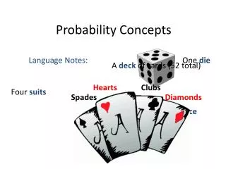
A Survey of Probability Concepts. Chapter 5. Modified by Boris Velikson, 2009. GOALS. Define probability. Describe the classical, empirical, and subjective approaches to probability. Explain the terms experiment, event, outcome, permutations, and combinations.

E N D
A Survey of Probability Concepts Chapter 5 Modified by Boris Velikson, 2009
GOALS • Define probability. • Describe the classical, empirical, and subjective approaches to probability. • Explain the terms experiment, event, outcome, permutations, and combinations. • Define the terms conditional probability and joint probability. • Calculate probabilities using the rules of addition and rules of multiplication. • Apply a tree diagram to organize and compute probabilities. • Calculate a probability using Bayes’ theorem.
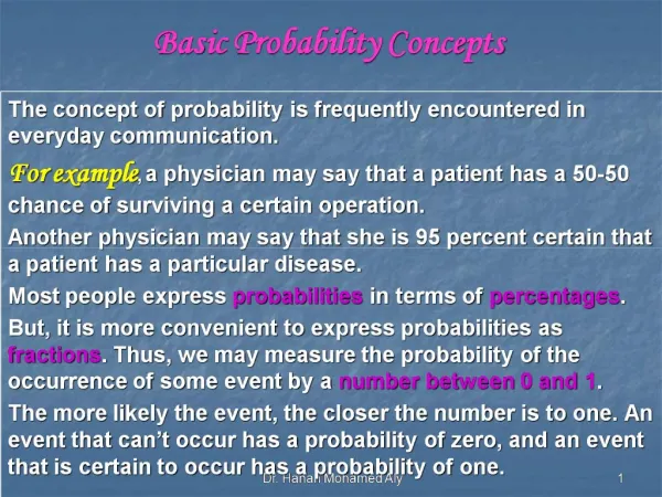
Definitions A probability is a measure of the likelihood that an event in the future will happen. It can only assume a value between 0 and 1. • A value near zero means the event is not likely to happen. A value near one means it is likely. • There are three ways of assigning probability: • classical, • empirical, and • subjective.
Definitions continued • An experimentis the observation of some activity or the act of taking some measurement. • An outcome is the particular result of an experiment. • An event is the collection of one or more outcomes of an experiment.
Assigning Probabilities Three approaches to assigning probabilities • Classical • Empirical • Subjective
Classical Probability Consider an experiment of rolling a six-sided die. What is the probability of the event “an even number of spots appear face up”? The possible outcomes are: There are three “favorable” outcomes (a two, a four, and a six) in the collection of six equally likely possible outcomes.
Mutually Exclusive Events • Events are mutually exclusive if the occurrence of any one event means that none of the others can occur at the same time. • Events are independent if the occurrence of one event does not affect the occurrence of another.
Collectively Exhaustive Events • Events are collectively exhaustive if at least one of the events must occur when an experiment is conducted.
Empirical Probability The empirical approach to probability is based on what is called the law of large numbers. The key to establishing probabilities empirically is that more observations will provide a more accurate estimate of the probability.
Law of Large Numbers Suppose we toss a fair coin. The result of each toss is either a head or a tail. If we toss the coin a great number of times, the probability of the outcome of heads will approach .5. The following table reports the results of an experiment of flipping a fair coin 1, 10, 50, 100, 500, 1,000 and 10,000 times and then computing the relative frequency of heads
Empirical Probability - Example On February 1, 2003, the Space Shuttle Columbia exploded. This was the second disaster in 113 space missions for NASA. On the basis of this information, what is the probability that a future mission is successfully completed?
Subjective Probability - Example • If there is little or no past experience or information on which to base a probability, it may be arrived at subjectively. • Illustrations of subjective probability are: 1. Estimating the likelihood the New England Patriots will play in the Super Bowl next year. 2. Estimating the likelihood you will be married before the age of 30. 3. Estimating the likelihood the U.S. budget deficit will be reduced by half in the next 10 years.
In-Class Exercises and HW • In class: Chapter 5 ex. 1,3,5,7,9 • HW: 2,4,6,8,10
Rules for Computing Probabilities Rules of Addition • Special Rule of Addition - If two events A and B are mutually exclusive, the probability of one or the other event’s occurring equals the sum of their probabilities. P(A or B) = P(A) + P(B) • The General Rule of Addition - If A and B are two events that are not mutually exclusive, then P(A or B) is given by the following formula: P(A or B) = P(A) + P(B) - P(A and B)
Addition Rule - Example What is the probability that a card chosen at random from a standard deck of cards will be either a king or a heart? P(A or B) = P(A) + P(B) - P(A and B) = 4/52 + 13/52 - 1/52 = 16/52, or .3077
Addition Rule - Remark But how do we calculate P(A and B) that we need to use the formula? In the last example we had a table that stated it explicitly. This is not always the case. The methods will be explained when we discuss Joint Probability on one of the next slides. The rule is simple when the events A and B are independent, more complicated otherwise.
The Complement Rule The complement rule is used to determine the probability of an event occurring by subtracting the probability of the event not occurring from 1. P(A) + P(~A) = 1 or P(A) = 1 - P(~A). (The notation ~A for “not A” is not the only one used. On also writes Ā, ┐ A, NOT A etc…)
In-Class Exercises and HW • In class: Self-Review exercise 5-3 (p.149) and nos. 11,13,17,21 • HW: 12,14,16,18,20,22
Joint Probability – Venn Diagram JOINT PROBABILITY A probability that measures the likelihood two or more events will happen concurrently.
Special Rule of Multiplication • The special rule of multiplication requires that two events A and B are independent. • Two events A and B are independentif the occurrence of one has no effect on the probability of the occurrence of the other. • This rule is written: P(A and B) = P(A)P(B)
Multiplication Rule-Example A survey by the American Automobile association (AAA) revealed 60 percent of its members made airline reservations last year. Two members are selected at random. What is the probability both made airline reservations last year? Solution: The probability the first member made an airline reservation last year is .60, written as P(R1) = .60 The probability that the second member selected made a reservation is also .60, so P(R2) = .60. Since the number of AAA members is very large, you may assume that R1 and R2 are independent. P(R1 and R2) = P(R1)P(R2) = (.60)(.60) = .36
Conditional Probability A conditional probability is the probability of a particular event occurring, given that another event has occurred. The probability of the event A given that the event B has occurred is written P(A|B).
General Multiplication Rule The general rule of multiplication is used to find the joint probability that two events will occur. Use the general rule of multiplication to find the joint probability of two events when the events are not independent. It states that for two events, A and B, the joint probability that both events will happen is found by multiplying the probability that event A will happen by the conditional probability of event B occurring given that A has occurred.
General Multiplication Rule - Example A golfer has 12 golf shirts in his closet. Suppose 9 of these shirts are white and the others blue. He gets dressed in the dark, so he just grabs a shirt and puts it on. He plays golf two days in a row and does not do laundry. What is the likelihood both shirts selected are white?
General Multiplication Rule - Example • The event that the first shirt selected is white is W1. The probability is P(W1) = 9/12 • The event that the second shirt selected is also white is identified as W2. The conditional probability that the second shirt selected is white, given that the first shirt selected is also white, is P(W2 | W1) = 8/11. • To determine the probability of 2 white shirts being selected we use formula: P(AB) = P(A) P(B|A) • P(W1 and W2) = P(W1)P(W2 |W1) = (9/12)(8/11) = 0.55
Contingency Tables A CONTINGENCY TABLE is a table used to classify sample observations according to two or more identifiable characteristics E.g. A survey of 150 adults classified each as to gender and the number of movies attended last month. Each respondent is classified according to two criteria—the number of movies attended and gender.
Contingency Tables - Example A sample of executives were surveyed about their loyalty to their company. One of the questions was, “If you were given an offer by another company equal to or slightly better than your present position, would you remain with the company or take the other position?” The responses of the 200 executives in the survey were cross-classified with their length of service with the company. What is the probability of randomly selecting an executive who is loyal to the company (would remain) and who has more than 10 years of service?
Contingency Tables - Example Event A1 happens if a randomly selected executive will remain with the company despite an equal or slightly better offer from another company. Since there are 120 executives out of the 200 in the survey who would remain with the company P(A1) = 120/200, or .60. Event B4 happens if a randomly selected executive has more than 10 years of service with the company. Thus, P(B4| A1) is the conditional probability that an executive who would remain with the company has more than 10 years of service. Of the 120 executives who would remain 75 have more than 10 years of service, so P(B4| A1) = 75/120. In fact, given a contingency table (not always given!), this could be read directly as (75/200).
Tree Diagrams A tree diagram is useful for portraying conditional and joint probabilities. It is particularly useful for analyzing business decisions involving several stages. A tree diagramis a graph that is helpful in organizing calculations that involve several stages. Each segment in the tree is one stage of the problem. The branches of a tree diagram are weighted by probabilities.
In-Class Exercises and HW • In class: Chapter 5 ex. 23,27,29,31 • HW: 24,26,28,30,32
Bayes’ Theorem – First, an example(pay attention - it is a LONG discussion!) • 5% of the population of Ulmen have a decease specific to that country. Events: A1 = “has the decease”; A2 = ~A1 = “doesn’t have the decease”. • We know: P(A1) = 0.05, P(A2) = 0.95 (these are called prior probabilities). • A diagnostic technique exists, but it is not very accurate: • If a person has the decease, the test shows it in 90% of cases (10% of “false negatives”). • If a person does not have the decease, the test is still positive in 15% of cases (15% of “false positives”). • Event: “Test positive” = B. • The conditional probabilities are: P(B|A1)=0.9, P(B|A2)=0.15 • We do not know: for a person randomly selected and testing positive, what is the probability he or she has the decease? - P(A1|B)=?
Bayes’ Theorem – Example, cont. • P(A1) = 0.05, P(A2) = 0.95, P(B|A1)=0.9, P(B|A2)=0.15 • Then what is P(A1|B)? It is the number of cases in which the person is sick, but out of the number of cases in which the test is positive, rather than out of the whole population. (See the contingency table below) • The problem is that we were not given P(A1 and B) and P(B).
Bayes’ Theorem – Example, cont. • Let us find P(A1 and B) and P(B). • According to the formula for joint probabilities, P(A1 and B)=P(A1)P(B|A1)=0.05×0.1=0.005. • To find P(B), we must argue. The number of times B happens is the sum of the numbers of times B happens and something else happens for the other variable, if these “something else’s” are mutually exclusive and collectively exhaustive (represent together all that can happen).
A1 A8 A2 A7 A3 A6 A4 A5 Bayes’ Theorem – Example, cont. • In fact, P(B)=P(B and A1)+ P(B and A2) . • In general, if there are more than 2 possibilities for the variable A, P(B)=ΣP(B and Ai) if Ai form a mutually exclusive and collectively exhaustive set. Why is it evident? • On this drawing, the rectangle represents “everything that can happen”. It is divided into 8 triangles representing events A1, A2, …, A8. They are mutually exclusive (they don’t intersect) and collectively exhaustive (together, they fill “everything”). The circle represents the event B. It can be thought of as a sum of 8 sectors: each sector is a combined event (B and A1) etc. B and A1
Bayes’ Theorem – Example, cont. • So, P(B)=P(B and A1)+ P(B and A2) • P(B and A1)=P(A1 and B)=P(A1)P(B|A1); • P(B and A2)=P(A2 and B)=P(A2)P(B|A2). • Therefore, P(B)=P(A1)P(B|A1)+P(A2)P(B|A2).
Bayes’ Theorem – Example, cont. We obtain Generalization: It follows from our discussion that if instead of two mutually exclusive and collectively exhaustive events A1 and A2 we had three (A1, A2, A3), the formula would read and so on.
Bayes’ Theorem, formulation (finally!) • Bayes’ Theorem is a method for revising a probability given additional information. • It is computed using the following formula : If there are two mutually exclusive and collectively exhaustive events A1 and A2. The generalization for three mutually exclusive and collectively exhaustive events A1, A2 and A3 is given on the previous slide. • Here P(A1) is called prior probability: the initial probability based on the present level of knowledge; • P(A1|B) is called posterior probability: a revised probability based on additional information.
Bayes’ Theorem – Example, reformulation. Let’s now fill the contingency table, where we’ll put in the cells the number of times an event is true (we could also use the probabilities). Let’s consider 10000 people. becomes first
Contingency Tables – a warning Be careful! A contingency table contains numbers out of a total, or probabilities of events and joint events, but not conditional probabilities! To obtain a conditional probability – say, P(A1|B) – you must divide the (A1 and B) entry by the B entry! (see next slide)
Bayes’ Theorem – Example, reformulation. So let’s calculate: The desired probability P(A1|B) is the ratio (450/1875)=0.24. We can see that in this case it is much simpler to use the contingency table than the Bayes’ formula. So why do we need the formula? Because it is more general and is more convenient if there is a large set of mutually exclusive and collectively exhaustive events.
Bayes’ Theorem – Example, summary of findings. The results can be summarized in the following table (it is NOT a contingency table!):