Download

1 / 36
370 likes | 1.12k Vues
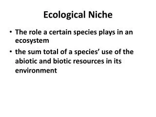
Ecological niche and ecological niche modeling. Tereza Jezkova School of Life Sciences, University of Nevada, Las Vegas March 2010. What drives species distributions?. All species have tolerance limits for environmental factors beyond which individuals cannot survive , grow , or reproduce.

E N D
Ecological niche and ecological niche modeling Tereza Jezkova School of Life Sciences, University of Nevada, Las Vegas March 2010
What drives species distributions? • All species have tolerance limits for environmental factors beyond which individuals cannot survive, grow, or reproduce
Environmental Gradient Tolerance Limits and Optimum Range Tolerance Limits Tolerance limits exist for all important environmental factors
Critical factors and Tolerance Limits • For some species, one factor may be most important in regulating a species’ distribution and abundance. • Usually, many factors interact to limit species distribution.
Critical factors and Tolerance Limits ? • Organism may have a wide range of tolerance to some factors and a narrow range to other factors
Specialist and Generalist species... Fig. 4-11, Miller & Spoolman 2009
FUNDAMENTAL NICHE Biotic factors Historical factors REALIZED NICHE Realized environment
Tolerance Limits and Optimum Range Fundamental versus realized niche Fundamental (theoretical) niche - is the full spectrum of environmental factors that can be potentially utilized by an organism Realized (actual) niche - represent a subset of a fundamental niche that the organism can actually utilize restricted by: - historical factors (dispersal limitations) - biotic factors (competitors, predators) - realized environment (existent conditions)
Tolerance Limits and Optimum Range Niche shift • Are niches stable? • Realized niche shifts all the time due to • changing biotic interations, • realized environment, • time to disperse NO! Time T1 Time T2 Realized Niche Shift
Fundamental niche shift when tolerance limits change due to evolutionary adaptation Time T1 Time T2 Fundamental Niche Shift
Resource Partitioning • Law of Competitive Exclusion - No two species will occupy the same niche and compete for exactly the same resources - Extinction of one of them - Niche Partitioning (spatial, temporal)
Niche partitioning and Law of Competitive Exclusion Chthamalus Balanus Chthamalus Balanus
Ecological niche modeling Purpose: · - Approximation of a Species Distribution
Ecological niche modeling Purpose: · - Potential Niche Habitat Modeling (Invasive species, diseases)
Ecological niche modeling Purpose: · - Site Selection or conservation priority: Suitability Analysis
Ecological niche modeling Purpose: · - Species Diversity Analysis
Ecological niche modeling Two types: 1. DEDUCTIVE: A priori knowledge about the organism Example: SWReGAP http://fws-nmcfwru.nmsu.edu/swregap/habitatreview/
Ecological niche modeling Two types: 2. CORRELATIVE: Self-learning algorithms based on known occurrence records and a set of environmental variables
Occurrence records: • Own surveys (small scale) • Digital Databases (e.g. museum specimens) • MANIS (mammals) • ORNIS (birds) • HERPNET (reptiles) • HAVE TO BE GEOREFERENCED (must have coordinates) http://manisnet.org/ http://olla.berkeley.edu/ornisnet/ http://www.herpnet.org/
WORLDCLIM http://worldclim.org/ • Variables: • Temperature (monthly) • Precipitation (monthly) • 19 Bioclimatic variables • Current, Future, Past • Resolution: • ca. 1, 5, 10 km • Coverage • World
Southwest Regional Gap Analysis Project http://earth.gis.usu.edu/swgap Northwest GAP Analysis Project http://gap.uidaho.edu/index.php/gap-home/Northwest-GAP • Variables: • Landcover • Resolution: • ca. 30 m • Coverage • western states
Natural Resources Conservation Service (NRCS) SSURGO Soil Data http://soils.usda.gov/survey/geography/ssurgo/ • Variables: • Soils • Resolution: • ca. 30 m • Coverage • USA but incomplete
Ecological niche modeling Step 1: occurrence records Step 2: environmental variables Step 3: current ecological niche Step 4: projected ecological niche
Problems: Models are only as good as the data that goes into it!!! • CALIBRATION MODELS • Insufficient or biased occurrence records • Insufficient or meaningless environmental variables • PROJECTION MODELS • Inaccuracies in climate reconstructions • Dispersal limitations • Non-analogous climates • Niche shift (evolution) !!! WRONG INTERPRETATIONS !!!
sasquatch blackbear
Exercise (work in pairs): • Download museum records for one of nine species • Prepare occurrence data file • Run the program Maxent for current (0K) and last glacial maximum (LGM) climate • Make maps in DivaGIS (or ArcGIS if you have it) • Answer questions on the worksheet • This PowerPoint is on the website, http://complabs.nevada.edu/~jezkovat/firefighters/niche_modelling.ppt so are the 0K and LGM datasets • Detailed instructions are at the end of this PowerPoint
Species: MAMMALS: Chisel-toothed kangaroo rat (Dipodomys microps) Desert kangaroo rat (Dipodomys deserti) Pygmy rabbit (Brachylagus idahoensis) Pika (Ochotona princeps) Mountain beaver (Aplodontia rufa) REPTILES and AMPHIBIANS: Desert Horned Lizard (Phrynosoma platyrhinos) Coastal Tailed Frog (Ascaphus truei) Long-nosed Leopard Lizard (Gambelia wislizenii) Gila monster (Heloderma suspectum)
Download Occurrence Records • Choose either Manis http://manisnet.org database (mammals) or Herpnet database http://www.herpnet.org/ (reptiles) • Select “Data portals” • In Manis, click on any of the three providers (e.g. MaNIS Portal at the Museum of Vertebrate Zoology • Click “build query” • Click “Arctos-MVZ catalog” and scroll down • Click on “select a concept” and choose “scientific name” • Click on “select a comparator” and choose “contains (% for wildcard) • Type in the scientific name (e.g. Dipodomys deserti) • Delete number under “Specify record limit” • Click on “submit query” • WAIT !!! • If the server crashes start over again ;) • When the server returns the result of your search, click on “Download tabular results” and save the file into a folder
Excel – prepare occurrence records csv. file • Open downloaded occurrence records in Excel (right-click and use the “open with” function • Delete unnecessary rows up front • Sort by “coordinate uncertainty” • Delete all records with no coordinates or those with coordinate uncertainty more than 5000 meters • Delete all columns except the species, latitude and longitude • Make sure the column representing the species has the same value in all cells • Format the columns representing latitude and longitude as numbers with 4 decimal places (Font – Format cells – Number – Number – 4 decimal places) • Save as “ .csv “
Maxent • Download the 0K and LGM bioclimatic variables http://complabs.nevada.edu/~jezkovat/firefighters/0K.ziphttp://complabs.nevada.edu/~jezkovat/firefighters/LGM.zip • Unzip each dataset into a separate folder • Open Maxent (*.bat file) • Import your *.csv file of occurrence records • Import the folder with the 0K bioclimatic variables • Check all three fields • Indicate the directory with the LGM layers • Indicate your output directory • Press “Run”
Diva GIS • Import your occurrence records by selecting: Data -> Import points to shapefile -> From text file (.txt) • Add the shapefile representing “states”: Layer –> add layer –> States.shp http://complabs.nevada.edu/~jezkovat/firefighters/states.zip (unzip first) • Import your 0K model generated by Maxent (your_species.asc) by selecting: Data -> Import to Gridfile ->Single file. Choose “ESRI ascii” of file and “select integer” • Repeat for your LGM model (your_species_ccsm.asc) • Use the zoom tool to zoom in or out to capture the model well • Unclick the LGM model • Click on “Design” in the bottom right corner and click “OK” in the top left corner • Save as *.bmp file • Click on “data” in the bottom right corner, unclick you OK model and check your LGM model. • Click on Design and repeat your steps as before
BIOCLIMATIC VARIABLES BIO1 = Annual Mean Temperature BIO2 = Mean Diurnal Range (Mean of monthly (max temp - min temp)) BIO3 = Isothermality (P2/P7) (* 100) BIO4 = Temperature Seasonality (standard deviation *100) BIO5 = Max Temperature of Warmest Month BIO6 = Min Temperature of Coldest Month BIO7 = Temperature Annual Range (P5-P6) BIO8 = Mean Temperature of Wettest Quarter BIO9 = Mean Temperature of Driest Quarter BIO10 = Mean Temperature of Warmest Quarter BIO11 = Mean Temperature of Coldest Quarter BIO12 = Annual Precipitation BIO13 = Precipitation of Wettest Month BIO14 = Precipitation of Driest Month BIO15 = Precipitation Seasonality (Coefficient of Variation) BIO16 = Precipitation of Wettest Quarter BIO17 = Precipitation of Driest Quarter BIO18 = Precipitation of Warmest Quarter BIO19 = Precipitation of Coldest Quarter