Ecological niche modeling: statistical framework
Ecological niche modeling: statistical framework. Miguel Nakamura Centro de Investigación en Matemáticas (CIMAT), Guanajuato, Mexico nakamura@cimat.mx Warsaw, November 2007. Niche modeling. “Data”. (Environment+ presences). +.


Ecological niche modeling: statistical framework
E N D
Presentation Transcript
Ecological niche modeling: statistical framework Miguel Nakamura Centro de Investigación en Matemáticas (CIMAT), Guanajuato, Mexico nakamura@cimat.mx Warsaw, November 2007
Niche modeling “Data” (Environment+ presences) + Neural networks, decision trees, genetic algorithms, maximum entropy, etc. “Model” “Prediction”
Ecological Niche Modeling: Statistical Framework • What is statistics? • Uncertainty and variation are omnipresent. • What is role of probability theory? • What is data? • What is a model? • Different goals that models try to achieve. • Different modeling cultures, sometimes confused or misunderstood. • What is a good model? • What is a statistical model? • Different needs for data. • Where do models come from?
What makes a model or method of analysis become statistical? • The layman’s view is that the statistical character comes merely from using observed empirical data as input. • The statistical profession tends to define it in terms of the tools used (e.g. probability models, Markov Chains, least-squares fitting, likelihood theory, etc.) • Example: “This chapter is divided into two parts. The first part deals with methods for finding estimators, and the second part deals with evaluating these (and other) estimators.” (Casella & Berger, Statistical Inference, 1990) • Some statistical thinkers suggest a much broader concept of statistics, based on the type of problems statistics attempts to solve. • Example: “Perhaps the subject of statistics ought to be defined in terms of problems, problems that pertain to analysis of data, instead of methods”. (Friedman, 1977)
The problem is statistical, not the model. • A statistical problem is characterized by: data subject to variability, a question of interest, uncertainty in the answer that data can provide, some degree of inferential reasoning required. • The convention is that subjects probability and statistics are studied together. Why? Because probability has two distinct roles in statistics: • To mathematically describe random phenomena, and • to quantify uncertainty of a conclusion reached upon analyzing data. • Why does the statistical profession stress certain types of methods? Because variation in statistical problems is recognized from the onset, and quantification of uncertainty is taken for granted and customarily addressed by such methods. Thus, one may understand a “statistical method” in the sense of assessing uncertainty. It is in this sense that some statisticians do not consider some data analyses to be “statistical” at all.
Modeler’s black box Y* X environment Prediction Model taxonomy Nature’s black box X Y environment Z Presence, absence (Y=0,1) other variables Why Y and Y* do not agree: (a) we do not know the black box, (b) we do not use Z, (c) We use X although Nature may not.
Modeler’s black box Y* X environment Prediction Use data to construct the inside of the black box. Hope that Y is close to Y* and that it holds for arbitrary values of X (this is validation, on Thursday) Modeler’s task Nature’s black box X Y environment Z Presence, absence (Y=0,1) other variables
For the modeler’s black box: two cultures* 1. Algorithmic Modeling (AM) culture 2. Data Modeling (DM) culture * Breiman (2001), Statistical Science, with discussion.
Algorithmic modeling culture Neural networks, decision trees, genetic algorithms, etc. • Inside of black-box complex and unknown. Interpretation often difficult. • Approach is to find a function f(x) (an algorithm). • Validation: examination of predictive accuracy. • Notion of uncertainty not necessarily addressed. Y*=f(X) X environment Prediction
Data modeling culture Logistic regression, linear regression, etc. • Probabilistic data model inside black box. This means assumptions regarding randomness, particularly facts known about the subject-matter at hand. • P(Y) (probability model for Y) is by-product (which in turn enables quantification of precision of prediction, e.g. Bayesian inference). • Parameters estimated via observed data. • Method of prediction prescribed by model and/or goals (also inside black box). • Validation: examination to determine if assumed randomness is explained. Term “goodness of fit” coined. Y*=E(Y|X) X environment Prediction
Illustrative example: simple linear regression Y X The difference between a data model and an algorithm.
Least squares fit based on probabilistic assumptions Y X X1 X2 X3
Data modeling viewpoint • Each observed Y is assumed to have a probability distribution (e.g. normal) for a given X. The linear structure is an assumption that may come from subject matter considerations (e.g. chemical theory). A probabilistic consideration (maximum likelihood) leads to the least squares fit. • As part of the fitting process, quantification of uncertainty in estimated parameters (slope and intercept) is obtained.
Least squares fit base on geometrical assumptions Y X X1 X2 X3
Algorithmic modeling viewpoint • There is no explicit role for probability. Points (X,Y) are merely approximated by a straight line. A geometrical (non-probabilistic) consideration (minimize a distance) also leads to the least squares fit. Slope and intercept not necessarily interpretable, nor of special interest. • Data model and algorithmic approach both yield least squares fit. Does this mean they are both doing the same thing and pursuing the same goals? No! For data model, line is estimate of probabilistic feature; for algorithmic model, line is an approximating device. • If only the fitted line is extracted from statistical analysis, the description of variability of Y (via the probability model) present in data modeling is completely disregarded!
If interest is value of Y at X0 Confidence intervals for Y ? X0 Quantification of uncertainty: conceived ad hoc for specific needs Y X
If interest is in the slope of function m(x)=b0+b1X ? Confidence intervals for b1 Quantification of uncertainty: conceived ad hoc for specific needs Y X
If interest is in the functionm(x)=E(Y|X) Confidence bands for m(x) ? Quantification of uncertainty: conceived ad hoc for specific needs Y X
Uncertainty X Y environment Z Presence, absence (Y=0,1) other variables If interest is in feasibility at the single site: should quantify uncertainty at that site. If interest is in feasibility at all the sites in the region: should quantify uncertainty of the resulting map.
What do we need a model for?a.k.a. What do we need a predicted distribution for? Explanation (needs some form of structural knowledge between variables). Decision-making (the map does not suffice; other criteria involved, such as costs). Prediction Classification All need some form of quantification of uncertainty. Inference Even it this did NOT include any uncertainty, it would still NOT fully provide answers to all questions. Hypothesis testing Estimation
Explanation or prediction? Inference or decision? • For explanation, Occam’s razor applies. A working model, a sufficiently good approximation that is simple is preferred. • For prediction, all that is important is that it works. Modern hardware+software+data base management have spawned methods from fields of artificial intelligence, machine learning, pattern recognition, and data visualization. • Depending on particular need, some models may not always provide the required answers.
Niche modeling complications • Missing data (presence-only; “pseudo-absences”) • Issues in scale • Spatial correlation • Quantity and quality of data • Curse of dimensionality • Multiple objectives • Subject matter considerations are extremely complex. • Massive amount of scenarios (Many species, many regions)
Summary of conclusions • The word “model” may have different meanings: Algorithmic modeling (AM) and data modeling (DM). • Prediction is important, but sometimes subject-matter understanding or decision-making is the ultimate goal. • Even if prediction IS the goal, it may be under different conditions than those applicable to data (e.g. niches under climate change, interactions). • Decision maker requires measure of uncertainty, in addition to description. • Purely empirical methods of general application also needed (e.g. data mining).
Note • GARP is algorithmic modeling culture. • Maxent is algorithmic modeling culture in its origin, but has a latent explanation in terms of the data modeling culture (Gibbs distribution and maximum likelihood).
Data modeling Algorithmic modeling DM vs. AM tradeoff
Summary of conclusions • “algorithms”, “data”, and “modeling” placed at different logical levels • In DM, algorithm is prescribed ad hoc as part of the black box; in AM it is the black box. • AM generally starts with data; DM generally starts with context and an issue, or a scientific hypothesis.
Summary of conclusions • Different “data” requirements by modelers from different modeling cultures • DM emphasizes context and underlying explanatory process a lot more, in addition to measured variables (why, how, in addition to where, when).
Some references • Cox, D.R. (1990), “Role of Models in Statistical Analysis”, Statistical Science, 5, 169–174. • Breiman, L. (2001), “Statistical Modeling: The Two Cultures”, Statistical Science, 16, 199–226. • Friedman, J.H. (1997), “Data Mining and Statistics: What’s the Connection?”, Department of Statistics and Stanford Linear Accelerator Center, Stanford University. • MacKay, R.J. and Oldford, R.W. (2000), “Scientific Method, Statistical Method, and the Speed of Light”, Statistical Science, 15, 224–253. • Ripley, B.D. (1993), “Statistical Aspects of Neural Networks”, in Networks and Chaos–Statistical and Probabilistic Aspects, eds. O.E. Barndorff-Nielsen, J.L. Jensen and W.S. Kendall, Chapman and Hall, 40–123. • Sprott, D. A. (2000), Statistical Inference in Science, Springer-Verlag, New York. • Argáez, J., Christen, J.A., Nakamura, M. and Soberón, J. (2005), “Prediction of Potential Areas of Species Distributions Based on Presence-only Data”, Journal of Environmental and Ecological Statistics, vol. 12, 27–44.