The Normal Distribution
The Normal Distribution. Mathematical models The Normal Distribution Introduction to Sampling Distributions. The Normal Distribution. Last class we talked about ways to describe distributions Central Tendency Variability

The Normal Distribution
E N D
Presentation Transcript
The Normal Distribution • Mathematical models • The Normal Distribution • Introduction to Sampling Distributions
The Normal Distribution • Last class we talked about ways to describe distributions • Central Tendency • Variability • Today we will talk about a theoretical distribution important in statistics • The Normal Distribution • The Ultimate Well-Behaved Distribution
Mathematical Models • Whenever we have a set of points, we might want to describe them with an equation. • This provides a formal description or model • When the set of points are observations from a sample, the model is a distribution • This model will smooth the curve from a histogram.
Why a model? • If the mathematical properties are known, then we can use this distribution to reason about the data. • For example, suppose we wanted to know whether a particular observation we obtained was common or extreme. • How would we know?
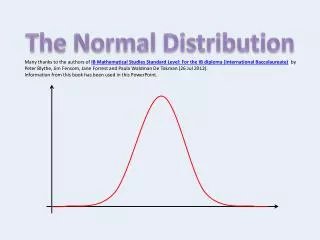
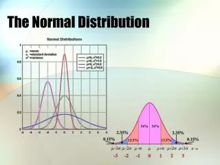
Using the Normal Distribution • The Normal distribution is one model distribution • It is defined by an equation that has 2 parameters that determine its shape • The Mean and the Standard Deviation
Different Normal Distributions • Changing the Mean Shifts the Distribution • Changing the Standard Deviation makes the distribution wider or narrower.
Area under the curve • Because the equation that specifies the distribution is known, we know the area under the curve. • The area under the curve is the proportion of observations that fall between those values. Mean=100, s.d. = 10
The standard Normal Distribution • All normal distributions are the same, except for a transformation. • We can change any observation into a standard score (sometimes called a z-score) • Z = (x-m)/s (m and s are population Mean and s.d.) Mean = 0 s.d. = 1
What is a z-score? • Using the z-score, you can find the proportion of observations as extreme or more extreme in the normal distribution • Just use your handy-dandy normal distribution chart. • Where do you get one? • Just open any statistics book, like, say, yours!
Practice with the z-scores • Suppose you are scouting for potential Olympic long jumpers. You observe 5000 sixth graders in the standing broad jump. • The distribution of the sample looks well-behaved • Mean = 6.53 feet • s.d. = 1.14 feet • What are the z-scores and probabilities for jumps of • 6.21 feet 6.53 feet • 4.38 feet 7.21 feet • 9.77 feet 3.11 feet
A return to sample size • So, how many people should you ask in a survey? • Imagine you want to know the average number of books read each year by everyone over the age of 10 in the United States. • What do you do? • Take a survey of N people, and calculate the mean of your sample. • You calculate the mean, because it is the best estimate of the population mean. • How good an estimate is it?
Sampling Distributions • The normal distribution can help. • If you survey N people, your survey will get some mean response X1. • If you took another survey of N people from the same population, this survey would have a mean X2. • If you took a bunch of surveys and plotted the means on a histogram, you would find something that looked like a normal distribution • Even if the data you are sampling is not normally distributed. • Sampling Distribution of the Mean
Lots of Means • This distribution of survey results would follow a normal distribution • Mean = • standard deviation = /(N)1/2 Sample N=5 Underlying Population Mean = 100 s.d. = 10 This is a distribution of means of samples of size N
Increasing sample size • As N (sample size) increases, the variability in this distribution decreases substantially. • By N = 1000, the true mean is quite likely to be very close to the mean obtained in the survey. Sample N = 1000 Sample N = 10
How big a sample? • The sampling distribution of the mean • Mean = • standard deviation = /(N)1/2 • As N gets larger, the standard deviation of the sampling distribution gets smaller. • Diminishing returns for additional observations • A cost-benefit analysis
Where will this return? • The normal distribution is a convenient mathematical construct, but it may not be a good model of your data. • Poorly behaved distributions deviate from the normal • The book provides ways to test the fit of a normal distribution to a set of data • The normal distribution will come back when we talk about inferential statistics later in the semester. • Many of the statistical tests we will talk about assume that the data being tested follow a normal distribution.

