Mining for Low Abundance Transcripts in Microarray Data
This study explores the challenges of detecting low abundance transcripts using microarray technology in the context of obesity and diabetes research. We address the limitations of differential gene expression analysis, including the role of genetic background, replication issues, and the high variability of low abundance signals. Data from various mouse genotypes, including lean and obese models, are analyzed to identify key genes and transcription factors influencing metabolic health. This research provides insights into the complex regulatory mechanisms underlying obesity.


Mining for Low Abundance Transcripts in Microarray Data
E N D
Presentation Transcript
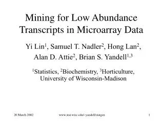
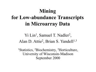
Mining for Low Abundance Transcripts in Microarray Data Yi Lin1, Samuel T. Nadler2, Hong Lan2, Alan D. Attie2, Brian S. Yandell1,3 1Statistics, 2Biochemistry, 3Horticulture, University of Wisconsin-Madison www.stat.wisc.edu/~yandell/statgen
Key Issues • differential gene expression using mRNA chips • diabetes and obesity study (biochemistry) • lean vs. obese mice: how do they differ? • what is the role of genetic background? • detecting genes at low expression levels • inference issues • formal evaluation of each gene with(out) replication • smoothly combine information across genes • significance level and multiple comparisons • general pattern recognition: tradeoffs of false +/– • modelling differential expression • gene-specific vs. dependence on abundance • R software module www.stat.wisc.edu/~yandell/statgen
Diabetes & Obesity Study • 13,000+ mRNA fragments (11,000+ genes) • oligonuleotides, Affymetrix gene chips • mean(PM) - mean(NM) adjusted expression levels • six conditions in 2x3 factorial • lean vs. obese • B6, F1, BTBR mouse genotype • adipose tissue • influence whole-body fuel partitioning • might be aberrant in obese and/or diabetic subjects • Nadler et al. (2000) PNAS www.stat.wisc.edu/~yandell/statgen
Low Abundance Genes for Obesity www.stat.wisc.edu/~yandell/statgen
Low Abundance Obesity Genes • low mean expression on at least 1 of 6 conditions • negative adjusted values • ignored by clustering routines • transcription factors • I-kB modulates transcription - inflammatory processes • RXR nuclear hormone receptor - forms heterodimers with several nuclear hormone receptors • regulation proteins • protein kinase A • glycogen synthase kinase-3 • roughly 100 genes • 90 new since Nadler (2000) PNAS www.stat.wisc.edu/~yandell/statgen
Obesity Genotype Main Effects www.stat.wisc.edu/~yandell/statgen
Low Abundance on Microarrays • background adjustment • remove local “geography” • comparing within and between chips • negative values after adjustment • low abundance genes • virtually absent in one condition • could be important: transcription factors, receptors • large measurement variability • early technology (bleeding edge) • prevalence across genes on a chip • up to 25% per chip (reduced to 3-5% with www.dChip.org) • 10-50% across multiple conditions • low abundance signal may be very noisy • 50% false positive rate even after adjusting for variance • may still be worth pursuing: high risk, high research return www.stat.wisc.edu/~yandell/statgen
Why not use log transform? • log is natural choice • tremendous scale range (100-1000 fold common) • intuitive appeal, e.g. concentrations of chemicals (pH) • looks pretty good in practice (roughly normal) • easy to test if no difference across conditions • but adjusted values = PM – MM may be negative • approximate transform to normal • very close to log if that is appropriate • handles negative background-adjusted values • approximate -1(F()) by -1(Fn()) www.stat.wisc.edu/~yandell/statgen
Normal Scores Procedure adjusted expression = PM – MM rank order R = rank() / (n+1) normal scores X = qnorm( R ) X = -1(Fn()) average intensity A = (X1+X2)/2 difference D = X1 – X2 variance Var(D | A) 2(A) standardization S = [D –(A)]/(A) www.stat.wisc.edu/~yandell/statgen
7. standardize S=D –center spread 0. acquire data PM,MM 1. adjust for background =PM – MM 2. rank order genes R=rank()/(n+1) 4. contrast conditions D=X1 –X2 A=mean(X) 3. normal scores X=qnorm(R) 5. mean intensity A=mean(X) www.stat.wisc.edu/~yandell/statgen
Robust Center & Spread • center and spread vary with mean expression X • partitioned into many (about 400) slices • genes sorted based on X • containing roughly the same number of genes • slices summarized by median and MAD • median = center of data • MAD = median absolute deviation • robust to outliers (e.g. changing genes) • smooth median & MAD over slices www.stat.wisc.edu/~yandell/statgen
Robust Spread Details • MAD ~ same distribution across A up to scale • MADi = i Si, Si ~ S, i = 1,…,400 • log(MADi ) = log(i) + log(Si), I = 1,…,400 • regress log(MADi) on Ai with smoothing splines • smoothing parameter tuned automatically • generalized cross validation (Wahba 1990) • globally rescale anti-log of smooth curve • Var(D|A) 2(A) • can force 2(A) to be decreasing www.stat.wisc.edu/~yandell/statgen
Anova Model • transform to normal: X = -1(Fn()) • Xijk = + Ci + Gj + (CG)ij + Ejjk • i=1,…,I conditions; j=1,…,J genes; k=1,…,K replicates • Ci = 0 if arrays normalized separately • Zi = 1(0) if (no) differential expression • Variance (Aj =jkXijk /IK) • Var(Xijk | Aj) = (Aj)2+ (Aj)2+ (Aj)2 if Zi = 1 • Var(Xijk | Aj) = (Aj)2+ (Aj)2 if Zi = 0 www.stat.wisc.edu/~yandell/statgen
Differential Expression • Djk = wi Xijk with wi = 0, wi2= 1 • Djk = wi (CG)ij + wi Ejjk • Variance depending on abundance • Var(Djk | Aj) = (Aj)2+ (Aj)2 if Zi = 1 • Var(Djk | Aj) = (Aj)2 if Zi = 0 • Variance depending on gene j ? • Var(Djk | j, Aj) = (Aj)2Vj, with Vj, ~ -1(,) • gene-specific variance • gene function-specific variance www.stat.wisc.edu/~yandell/statgen
gene-specific variance? www.stat.wisc.edu/~yandell/statgen
Bonferroni-corrected p-values • standardized differences • Sj= [Dj–(Aj)]/(Aj) ~ Normal(0,1) ? • genes with differential expression more dispersed • Zidak version of Bonferroni correction • p = 1 – (1 – p1)n • 13,000 genes with an overall level p = 0.05 • each gene should be tested at level 1.95*10-6 • differential expression if S > 4.62 • differential expression if |Dj–(Aj)| > 4.62(Aj) • too conservative? weight by Aj? • Dudoit et al. (2000) www.stat.wisc.edu/~yandell/statgen
comparison of multiple comparisons uniform j/(1+n)grey p-value black nominal .05 red Holms purple Sidak blue Bonferroni www.stat.wisc.edu/~yandell/statgen
Patterns of Differential Expresssion • (no) differential expression: Z = (0)1 • Sj|Zj ~ density fZ • f0 = standard normal • f1 = wider spread, possibly bimodal • Sj ~ density f = (1 – 1)f0 +(1 – 1)f1 • chance of differential expression: 1 • prob(Zj = 1) = 1 • prob(Zj = 1 | Sj ) = 1 f1(Zj) / f(Zj) www.stat.wisc.edu/~yandell/statgen
density of standardized differences • S =[D –(A)]/(A) • f = black line • standard normal • f0 = blue dash • differential expression • f1 = purple dash • Bonferroni cutoff • vertical red dot www.stat.wisc.edu/~yandell/statgen
Looking for Expression Patterns • differential expression: D = X1 – X2 • S = [D –center]/spread ~ Normal(0,1) ? • classify genes in one of two groups: • no differential expression (most genes) • differential expression more dispersed than N(0,1) • formal test of outlier? • multiple comparisons issues • posterior probability in differential group? • Bayesian or classical approach • general pattern recognition • clustering / discrimination • linear discriminants (Fisher) vs. fancier methods www.stat.wisc.edu/~yandell/statgen
Related Literature • comparing two conditions • log normal: var=c(mean)2 • ratio-based (Chen et al. 1997) • error model (Roberts et al. 2000; Hughes et al. 2000) • empirical Bayes (Efron et al. 2002; Lönnstedt Speed 2001) • gene-specific Dj ~ , var(Dj) ~-1, Zj ~ Bin(p) • gamma • Bayes (Newton et al. 2001, Tsodikov et al. 2000) • gene-specific Xj ~, Zj ~ Bin(p) • anova (Kerr et al. 2000, Dudoit et al. 2000) • log normal: var=c(mean)2 • handles multiple conditions in anova model • SAS implementation (Wolfinger et al. 2001) www.stat.wisc.edu/~yandell/statgen
R Software Implementation • quality of scientific collaboration • hands on experience of researcher • save time of stats consultant • raise level of discussion • focus on graphical information content • needs of implementation • quick and visual • easy to use (GUI=Graphical User Interface) • defensible to other scientists • public domain or affordable? • www.r-project.org www.stat.wisc.edu/~yandell/statgen
library(pickgene) ### R library library(pickgene) ### create differential expression plot(s) result <- pickgene( data, geneID = probes, renorm = sqrt(2), rankbased = T ) ### print results for significant genes print( result$pick[[1]] ) ### density plot of standardized differences pickedhist( result, p1 = .05, bw = NULL ) www.stat.wisc.edu/~yandell/statgen