Download
1 / 1
40 likes | 229 Vues
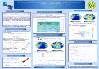
Three-dimensional Reconstruction of Ionosphere/ Plasmasphere using GNSS measurements Alizadeh M.M. (1), 2 , Schuh H. 1, 2 , Schmidt M. 3 Research Group Advanced Geodesy, Department of Geodesy and Geoinformation , Vienna University of Technology, Austria

E N D
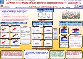
Three-dimensional Reconstruction of Ionosphere/Plasmasphereusing GNSS measurements • Alizadeh M.M. (1), 2, Schuh H.1,2, Schmidt M.3 • Research Group Advanced Geodesy, Department of Geodesy and Geoinformation, Vienna University of Technology, Austria • Department of Geodesy and GeoinformationScience, Technical University of Berlin, Berlin, Germany • DeutschesGeodätischesForschungsinstitut (DGFI), Munich, Germany • alizadeh@mail.tuwien.ac.at zero-degree SH coefficients and 6. Results predefined height range small numerical constant geomagnetic latitude local time 1. Introduction 4. Simulating input data Figures below depict estimated results for the snap-shot at [0,2] UT, day 182, 2010. (7) VTEC values for all IPP of GNSS observations are extracted from IGS VTEC maps. Fig. 5(a) Estimated maximum electron density ( ×1011elec/m3) and (b) estimated maximum electron density height (km) GNSS estimated model, doy 182, 2010 – [0,2]UT To illustrate a better understanding of the estimated parameters, the related Nm and hm values are depicted in a 3D conjunction plot: 2. TEC observable and Chapman function As an experimental step, we simulate the input data. Since STEC in Eq. (1) is related to VTEC using a mapping function F(z’) where z‘ is the satellite zenith angle at the Ionosphere Pierce Point (IPP). The additional terms in Eq. (5) could be neglected when using simulated data, so the relation would be simplified to (6) Fig. 3 – input data with true GNSS ray-path, but simulated values from IGS GIM (1) 5. Estimation Procedure (2) • Calculating a priori values Fig. 6 – 3D model of F2-peak electron density for day 182, 2010 - [0,2]UT; color bar indicates the maximum electron density (x1011 elec/m3) and the Z-axis indicates maximum electron density height in km Calculated using IRI-2012 Simulated using IGS VTEC Calculated using ray-tracing (8) 7. Conclusions and Outlook (3) (9) where • This study: • is pioneer in modeling the upper atmosphere, using space geodetic techniques, • includes geophysical parameters, i.e. F2-peak electron density and its corresponding height, • provides information about the ionosphere at different altitudes. • Our further steps are: • Applying real GNSS observations, • Integrating data from different space geodetic techniques, • Taking curvature effect and higher-order ionospheric effects into account, using ray-tracing technique, • Estimating plasmaspheric parameters as well as characteristic parameters of other layers as individual unknowns, • 4D modeling of electron density applying Fourier series expansion. • References • Alizadeh M. Multi-dimensional modeling of the ionospheric parameters, using space geodetic techniques, Ph.D. thesis, Vienna University of Technology, February 2013, in press. • FeltensJ., Chapman Profile Approach for 3-D Global TEC Representation., Proceedings of the 1998 IGS Analysis Workshop, ESOC, Darmstadt, Germany, February 1998. Substituting electron density from Eq. (3) into TEC observable Eq. (2) and Eq.(1),we obtain the relation between TEC observable and electron density: (4) Figure 4 – (a) Maximum electron density (elec/m3), and (b) maximum electron density height (km) from IRI background model, doy 182, 2010 – [0,2] UT • Representing unknown parameters with spherical harmonics Fig.1 – Expressing electron density with Chapman function 3. Ray-tracing technique To solve the integral in Eq. (4) numerically, a ray-tracing technique is deployed. Using this technique the values for satellite zenith angle, solar zenith angle, height increment at each layer, and height of layer above the Earth’s surface can be determined. So the integration in Eq. (4) will turn into a simple summation: • Applying constraints • Global mean constraint (for estimating Nm and hm) • Surface function (for estimating Nm) (Feltens et al. 2010) (10) (11) Fig.2 – Curved and straight ray-paths (12) Acknowledgement (5) The project MDION (P22203-N22) is funded by the Austrian Science Fund (FWF) EGU General Assembly 2013, 7 – 12 April 2013, Vienna, Austria In Eq. (5) plasmaspheric contribution is neglected and only bottom-side ionosphere is presented.