PID Controllers
PID Controllers. Gang Zhou. University of Virginia February 2006. I Control: Integral Control PI Control: Proportional-Integral Control PD Control: Proportional-Derivative Control PID Control: Proportional-Integral-Derivative Control Summary. Outline. Introducing I Control.

PID Controllers
E N D
Presentation Transcript
PID Controllers Gang Zhou University of Virginia February 2006
I Control: Integral Control PI Control: Proportional-Integral Control PD Control: Proportional-Derivative Control PID Control: Proportional-Integral-Derivative Control Summary Outline
Introducing I Control • What is wrong with P control? • Non-zero steady-state error • Prove it • A real CS case
Introducing I Control • What is I control? • The controller output is proportional to the integral of all past errors
Steady-State Error with I Control • Start from Example 9.1: the IBM Lotus Domino Server
More General • The steady-state error of a system with I control is 0, as long as the close-loop system is stable.
Transient Response with I Control • I Control eliminates the steady-state error, but it slows the system down • The reason is the added open-loop pole 1, which generates a close-loop pole that is usually close to 1. • Example 9.2: Closed-loop poles of the IBM Lotus Domino Server
Example 9.2 (continue) • Observe the root locus • The largest closed-loop pole is always closer to the unit circle than the open-loop pole 0.43.
Example 9.3 • Disturbance Rejection in the IBM Lotus Domino Server
Example 9.4 • Moving-average filter plus I control • A moving average slows down the system responses • An I control also slows down the system response • So the combination leads to undesirable slow behavior • Example: IBM Lotus Domino server + I control + Moving-average filer
Moving-average filter vs. I controller • An I controller works like a moving-average filter: • More response to sustained change in the output than a short transient disturbance • An I controller drives the steady-state error to 0, but the moving-average filter does not.
Steady-state Error with PI Control • PI has a zero steady-state error, in response to a step change in the reference input • It also holds for the disturbance input
PI Control Design by Pole Placement • Design Goals: • Assumption: G(z) is a first-order system • A higher-order system is approximated by a first-order system (chapter 3)
PI Control Design by Pole Placement • Approaches: • Step 1: compute the desired closed-loop poles • Step 2,3,4: find the P control gain and I control gain • Step 5: Verify the result • Check that the closed-loop poles lie within the unit circle • Simulate transient response to assess if the design goals are met
PI Control Design by Pole Placement • Example 9.5: Consider the IBM Lotus Domino server
Example 9.5 (continue) P control leads to quicker response I control leads to 0 steady-state error
PI Control Design Using Root Locus • The new issue: • The root locus allows only one parameter to be varied • A PI controller has two parameters: • The P control gain, and the I control gain • Solution to this issue: • Determine possible locations of the PI controller’s zero, relative to other poles and zeros • For each relative location of the zero, draw the root locus • For the most promising relative locations, try a few possible exact locations • Simulate to verify the result
PI Control Design Using Root Locus • Example 9.6: PI control using root locus
Example 9.6 (continue) P control leads to quicker response I control leads to zero steady-state error
CHR Controller Design Method • Example 9.7:
Example 9.7 (continue) • No simulation is needed to verify it. Why? - Only one option in the table
D Control • A Real CS Example: • An IBM Lotus Domino server is used for healthy consulting. (MaxUsr, RIS) • Bird flu happens in this area. More and more people request for the service. • More and more hardware is added to the server. • So the reference point keeps increasing. • To deal with the increasing reference point, do we have better choices than P/I control? • How about setting the control output proportional to the rate of error change?
D Control • D Control: the control output is proportional to the rate of change of the error • D control is able to make an adjustment prior to the appearance of even larger errors. • D control is never used alone, because of its zero output when the error remains constant. • The steady-state gain of a D control is 0.
PD Control • PD controllers are not appropriate for first-order systems because pole placement is quite limited • PD controllers can be used to reduce the overshoot for a system that exhibits a significant amount of oscillation with P control • Example: consider a second-order system
It sounds good It is real good Example (continue)
PID Control • PI controllers are preferred over PID controller • D control is sensitive to the stochastic variations • A low-pass filter can be applied to smooth the system output. In that case, the D control only responds to large changes • But the filter slows down the system response • PID Control Design by Pole placement • Compute the dominant poles based on the design goals • Compute the desired characteristic polynomial • Compute the modeled characteristic polynomial • Solve for the gains of the P, I and D control by coefficient matching • Verify the result
PID control design by pole placement • Example 9.8: • Consider the IBM Lotus Domino Server
Summary • I control adjust the control input based on the sum of the control errors • Eliminate steady-state error • Increase the settling time • D control adjust the control input based on the change in control error • Decrease settling time • Sensitive to noise • P, I and D can be used in combination • PI control, OD control, PID control
Summary (continue) • Pole placement design • Find the values of control parameters based on a specification of desired closed-loop properties. • Root locus design • Observe how closed-loop poles change as controller parameters are adjusted • Empirical method: • The values of control parameters can be determined by empirical methods based on the step response of the open-loop system