Random Variable and its Properties

1. Random Variable and its Properties Prof. Dr. S. K. Bhattacharjee Department of Statistics University of Rajshahi

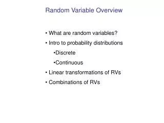
2. Random Variable and its Properties • Basic concepts, Discrete and Continuous random variables, Density and Distribution functions, Mathematical expectations and Variance, Functions of a random variable. Marginal and Conditional distributions. Conditional expectation and conditional variance. Conditional independence, Entropy.

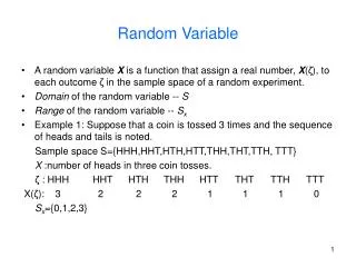
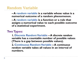
3. Random Variable • Let Ω be a sample space corresponding to some experiment ξ and let X: Ω→ R be a function from the sample space to the real line. Then X is called a random variable. • A random variable is a function from a sample space into the real numbers. • the outcome of the experiment is a random variable

4. Examples of Random Variables

5. Discrete and Continuous R.V.

6. Examples of Discrete R.V. • No. of students attending in a class. • No. of accident in a particular day. • No. of mobile calls in an hour.

7. Examples of Continuous R.V. • Height of a man. • Amount of water drinks a person per day. • Amount of rice consumption of a family per month.

8. Probability Distribution • Since Random variables cannot be predicted exactly, they must be described in the language of probability. • Every outcome of the experiment will have a probability associated with it. • The pattern of probabilities that are assigned to the values of the random variable is called the probability distribution of the random variable. • Two types of Distribution: Discrete Distribution and Continuous Distribution.

9. Probability Distributions of Discrete Random Variables The probability distribution of a discrete random variable Y is the set of values that this random variable can take, together with their associated probabilities. Probabilities are numbers between zero and one inclusive that always add to one when summed over all possible values of the random variable. Example: If we toss a fair coin twice, and Y is the total number of heads that turn up. Probability Distribution of Y is

10. Probability Distribution and CDF Mathematical form of this distribution is Pr{y=x}= The CDF is defined by F(x)= Pr{Y≤x} =

11. Graph of CDF for Discrete Distribution

12. Example

13. Probability Distribution and CDF

14. Density Functions of Binomial and Poisson Distributions.

15. Examples of Discrete Probability Distribution • Bernoulli • Binomial • Poisson • Negative Binomial • Uniform • Hypergeometric

16. Density Function for Continuous Random Variables

17. Density Function and CDF for Continuous R.V.

18. Density Function for Continuous Random Variables

19. Examples of Continuous Distribution • Uniform • Normal • Exponential • Gamma • Beta

20. Normal Probability Distribution The pdf of this distribution is given by

21. Density Curve of Normal Distribution

22. Example of Normal Distribution

23. Answer

24. Answer

25. Answer

26. Answer

27. Expectations of Random Variables

28. Variance of R.V.

29. Example Consider as an example the New York State Daily Numbers lottery game. The simplest version of the game works as follows: each day a three digit number between 000 and 999, inclusive, is chosen. You pay $1 to bet on a particular number in a game. If your umber comes up, you get back $500 (for a net profit of $499), and if your number doesn’t come up, you get nothing (for a net loss of $1). Consider the random process that corresponds to one play of the game, and define the random variable W to be the net winnings from a play. The following table summarizes the properties of the random variable as they relate to the random process: Outcome of process Probability Value of W Your number comes up p = 1/1000 W = 499 Your number doesn’t come up p = 999/1000 W = −1

30. Mean In the long run, we expect to win 1 time out of every 1000 plays, where we’d win $499, and we expect to lose 999 out of every 1000 plays, where we’d lose $1 (this is just the frequency theory definition of probabilities). That is, our rate of winnings per play, in the long run, would be $499, .001 of the time, and −$1, .999 of the time, or (499)(.001) + (−1)(.999) = −.5. In the long run, we lose 50/c each time we play. Note that on any one play, we never lose 50/c (we either win $499 or lose $1); rather, this is saying that if you play the game 10000 times, you can expect to be roughly $5000 down at the end. An even better way to look at it is that if 10 million people play the game every day, the state can expect to only have to give back about $5 million, a daily profit of a cool $5 million (this is why states run lotteries!).

31. Variance

32. Examples

33. Expectations of Functions of Random Variable

34. Properties of Expectations

35. Properties of Expectations

36. Properties of Expectations

37. Joint Probability Mass Function

38. Marginal Distribution

39. Conditional Distribution

40. Conditional Variance

41. Marginal and Conditional Distribution

42. Conditional Mean and Variance • Marginal Distribution of X: X : 0 1 2 P(X) : ¼ ½ ¼ • Conditional Distribution of X given Y = 1: X : 0 1 2 P(X|Y=1) : ¼ ½ ¼ E(X|Y=1) = 0x1/4 + 1x1/2 + 2x1/4 = 1 E(X2|Y=1) = 02x1/4 +12 x1/2 +22 x1/4 = 3/2 V(X|Y=1) = E(X2|Y=1) - {E(X|Y=1)}2 = 1/2

43. Conditional Density and Conditional Expectation of Continuous R.V.

44. Conditional Density of Continuous R.V.

45. Conditional Variance of Continuous R.V.

46. Marginal and Conditional Distribution for Continuous R.V.

47. Conditional Mean and Variance for Continuous R.V

48. Independence of R.V.

49. Entropy

50. Conditional Entropy