Download

1 / 56
560 likes | 655 Vues
Explore K-Means clustering algorithm, convergence, seed choice, and time complexity. Presentation details and example included. Learn to evaluate results and solutions to seed initialization problems.

E N D
Announcements • end of next class (May 19), at 8:45, take-home finals will be given. • Due: May 26 at 6 PM • project presentation – more in the next slide • project report due: May 26 at the time of presentation.
Project Presentation – Details • recommended format: slides with overhead projector (e.g. power-point) • sample presentations – e-mailed and can be found under project link • duration: 15 minutes • should include: • Problem statement • Data set – size, how acquired, processing needed • Algorithm – overview, time and space needs • Result – performance, plots • Challenges • Summary and conclusion
Sec. 16.4 K-Means • Assumes documents are real-valued vectors. • Clusters based on centroids (aka the center of gravity or mean) of points in a cluster, c: • Reassignment of instances to clusters is based on distance to the current cluster centroids.
Sec. 16.4 K-Means Algorithm Select K random docs {s1, s2,… sK} as seeds. Until clustering converges (or other stopping criterion): for each doc di: Assign di to the cluster cjsuch that dist(xi, sj) is minimal. (Next, update the seeds to the centroid of each cluster) for each cluster cj sj= (cj)
Sec. 16.4 Pick seeds Reassign clusters Compute centroids Reassign clusters x x Compute centroids x x x x K Means Example(K=2) Reassign clusters Converged!
Sec. 16.4 Termination conditions • Several possibilities, e.g., • A fixed number of iterations. • Doc partition unchanged. • Centroid positions don’t change. Does this mean that the docs in a cluster are unchanged?
Sec. 16.4 Convergence • Why should the K-means algorithm ever reach a fixed point? • A state in which clusters don’t change. • K-means is a special case of a general procedure known as the Expectation Maximization (EM) algorithm. • EM is known to converge. • Number of iterations could be large. • But in practice usually isn’t
Sec. 16.4 Convergence of K-Means • Define goodness measure of cluster k as sum of squared distances from cluster centroid: • Gk = Σi (di – ck)2 (sum over all di in cluster k) • G = Σk Gk • Reassignment monotonically decreases G since each vector is assigned to the closest centroid.
Sec. 16.4 Convergence of K-Means • Recomputation monotonically decreases each Gksince (mk is number of members in cluster k): • Σ (di – a)2 reaches minimum for: • Σ –2(di – a) = 0 • Σ di = Σ a • mK a = Σ di • a = (1/ mk) Σ di = ck • K-means typically converges quickly
Sec. 16.4 Time Complexity • Computing distance between two docs is O(M) where M is the dimensionality of the vectors. • Reassigning clusters: O(KN) distance computations, or O(KNM). • Computing centroids: Each doc gets added once to some centroid: O(NM). • Assume these two steps are each done once for I iterations. • Total time = O(IKNM). However, it is not clear how to bound I unless it is forced externally.
Sec. 16.4 Seed Choice • Results can vary based on random seed selection. • Some seeds can result in poor convergence rate, or convergence to sub-optimal clusters. • Select good seeds using a heuristic (e.g., doc least similar to any existing mean) • Try out multiple starting points • Initialize with the results of another method. Example showing sensitivity to seeds In the above, if you start with B and E as centroids you converge to {A,B,C} and {D,E,F} If you start with D and F you converge to {A,B,D,E} {C,F}
Two different K-means Clusterings Optimal Clustering Sub-optimal Clustering Original Points
Problem with Selecting Initial centroids If there are K ‘real’ clusters then the chance of selecting one centroid from each cluster is small. Chance is relatively small when K is large If clusters are the same size, n, then For example, if K = 10, then probability = 10!/1010 = 0.00036 Sometimes the initial centroids will readjust themselves in ‘right’ way, and sometimes they don’t
Solutions to Initial Centroids Problem Multiple runs Helps, but probability is not on your side Sample and use hierarchical clustering to determine initial centroids Select more than k initial centroids and then select among these initial centroids Select most widely separated Postprocessing Bisecting K-means Not as susceptible to initialization issues
Evaluating K-means Clusters Most common measure is Sum of Squared Error (SSE) For each point, the error is the distance to the nearest cluster To get SSE, we square these errors and sum them. x is a data point in cluster Ci and mi is the representative point for cluster Ci can show that micorresponds to the center (mean) of the cluster Given two clusters, we can choose the one with the smallest error One easy way to reduce SSE is to increase K, the number of clusters A good clustering with smaller K can have a lower SSE than a poor clustering with higher K
Sec. 16.4 K-means: issues, variations, etc. • Recomputing the centroid after every assignment (rather than after all points are re-assigned) can improve speed of convergence of K-means. • Assumes clusters are spherical in vector space • Sensitive to coordinate changes, weighting etc. • Disjoint and exhaustive • Doesn’t have a notion of “outliers” by default • But can add outlier filtering
How Many Clusters? • Number of clusters K is given • Partition n docs into predetermined number of clusters • Finding the “right” number of clusters is part of the problem • Given docs, partition into an “appropriate” number of subsets. • E.g., for query results - ideal value of K not known up front - though UI may impose limits. • Can usually take an algorithm for one flavor and convert to the other.
K not specified in advance • Say, the results of a query. • Solve an optimization problem: penalize having lots of clusters • application dependent, e.g., compressed summary of search results list. • Tradeoff between having more clusters (better focus within each cluster) and having too many clusters
K not specified in advance • Given a clustering, define the benefit for a doc to be the cosine similarity to its centroid. • Define the total benefit to be the sum of the individual doc benefits.
Penalize lots of clusters • For each cluster, we have a Cost C. • Thus for a clustering with K clusters, the Total Cost is KC. • Define the Value of a clustering to be = Total Benefit - Total Cost. • Find the clustering of highest value, over all choices of K. • Total benefit increases with increasing K. But can stop when it doesn’t increase by “much”. The Cost term enforces this.
Pre-processing and Post-processing Pre-processing Normalize the data Eliminate outliers Post-processing Eliminate small clusters that may represent outliers Split ‘loose’ clusters, i.e., clusters with relatively high SSE Merge clusters that are ‘close’ and that have relatively low SSE Can use these steps during the clustering process
Limitations of K-means: Non-globular Shapes Original Points K-means (2 Clusters)
Overcoming K-meansLimitations Original Points K-means Clusters • One solution is to use many clusters. • Find parts of clusters, but need to put together.
Overcoming K-means Limitations Original Points K-means Clusters
Overcoming K-means Limitations Original Points K-means Clusters
Ch. 17 animal vertebrate invertebrate fish reptile amphib. mammal worm insect crustacean Hierarchical Clustering • Build a tree-based hierarchical taxonomy (dendrogram) from a set of documents. • One approach: recursive application of a partitional clustering algorithm.
Dendrogram: Hierarchical Clustering • Clustering obtained by cutting the dendrogram at a desired level: each connected component forms a cluster.
Sec. 17.1 Hierarchical Agglomerative Clustering • Starts with each doc in a separate cluster • then repeatedly joins the closest pair of clusters, until there is only one cluster. • The history of merging forms a binary tree or hierarchy.
Sec. 17.2 Closest pair of clusters • Many variants to defining closest pair of clusters • Single-link • Similarity of the most cosine-similar (single-link) • Complete-link • Similarity of the “furthest” points, the least cosine-similar • Centroid • Clusters whose centroids (centers of gravity) are the most cosine-similar • Average-link • Average cosine between pairs of elements
Sec. 17.2 Single Link Agglomerative Clustering • Use maximum similarity of pairs: • Can result in “straggly” (long and thin) clusters due to chaining effect. • After merging ci and cj, the similarity of the resulting cluster to another cluster, ck, is:
Sec. 17.2 Single Link Example
Sec. 17.2 Complete Link • Use minimum similarity of pairs: • Makes “tighter,” spherical clusters that are typically preferable. • After merging ci and cj, the similarity of the resulting cluster to another cluster, ck, is: Ci Cj Ck
Sec. 17.2 Complete Link Example
Sec. 17.2.1 Computational Complexity • In the first iteration, all HAC methods need to compute similarity of all pairs of N initial instances, which is O(N2). • In each of the subsequent N2 merging iterations, compute the distance between the most recently created cluster and all other existing clusters. • In order to maintain an overall O(N2) performance, computing similarity to each other cluster must be done in constant time. • Often O(N3) if done naively or O(N2log N) if done more cleverly
Sec. 17.3 Group Average • Similarity of two clusters = average similarity of all pairs within merged cluster. • Compromise between single and complete link. • Two options: • Averaged across all ordered pairs in the merged cluster • Averaged over all pairs between the two original clusters • No clear difference in efficacy
Sec. 17.3 Computing Group Average Similarity • Always maintain sum of vectors in each cluster. • Compute similarity of clusters in constant time:
Sec. 16.3 What Is A Good Clustering? • Internal criterion: A good clustering will produce high quality clusters in which: • the intra-class (that is, intra-cluster) similarity is high • the inter-class similarity is low • The measured quality of a clustering depends on both the document representation and the similarity measure used
Sec. 16.3 External criteria for clustering quality • Quality measured by its ability to discover some or all of the hidden patterns or latent classes in gold standard data • Assesses a clustering with respect to ground truth. (requires labeled data) • Assume documents with C gold standard classes, while our clustering algorithms produce K clusters, ω1, ω2, …, ωK with nimembers.
Sec. 16.3 External Evaluation of Cluster Quality • Simple measure: purity, the ratio between the dominant class in the cluster πi and the size of cluster ωi • Biased because having n clusters maximizes purity • Others are entropy of classes in clusters (or mutual information between classes and clusters)
Sec. 16.3 Purity example Cluster I Cluster II Cluster III Cluster I: Purity = 1/6 (max(5, 1, 0)) = 5/6 Cluster II: Purity = 1/6 (max(1, 4, 1)) = 4/6 Cluster III: Purity = 1/5 (max(2, 0, 3)) = 3/5
Sec. 16.3 Rand Index measures between pair decisions Here RI = 0.68
Sec. 16.3 Rand index and Cluster F-measure Compare with standard Precision and Recall: People also define and use a cluster F-measure, which is probably a better measure.