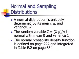
Normal Distribution in Statistics
380 likes | 478 Vues
Explore the history, function rule, and areas under the normal distribution, converting scores to z-scores, and interpreting test scores in terms of percentile ranks and standard scores.

Normal Distribution in Statistics
E N D
Presentation Transcript
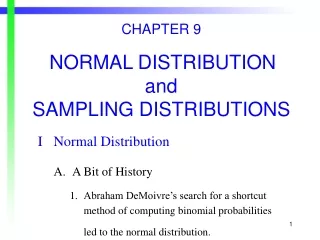
CHAPTER 9 NORMAL DISTRIBUTION and SAMPLING DISTRIBUTIONS I Normal Distribution A. A Bit of History 1. Abraham DeMoivre’s search for a shortcut method of computing binomial probabilities led to the normal distribution.
Figure 1. Normal distribution superimposed on the probability distribution for tossing 16 fair coins. As the number, n, of coins increases, the correspondence between the normal distribution and the binomial distribution becomes better and better.
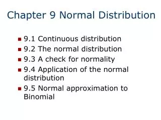
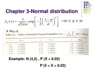
B. Function Rule for the Normal Distribution 1. The height of the distribution, f(X), is given by where and 2 identify a particular normal distribution is approximately 3.1416 e is approximately 2.718
C. Finding Areas under the Standard Normal Distribution Using Appendix Table D.2 1. Converting scores, X, to standard scores, z scores,
2. z scores have a mean = 0 and a standard deviation = 1. The mean and standard deviation are the same as the mean and standard deviation of the standard normal distribution. 3. Example of a z score transformation Consider a raw score of X = 123.5, where
Table 1 Areas under the standard normal distribution (From Appendix Table D.2)
4. Areas corresponding to columns 2 and 3 of the standard normal distribution table Figure 2. The subscript denotes the size of the area that lies above the z score.
5. Using the standard normal distribution to find the raw score corresponding to a percentile rank distributed, the raw score corresponding to the 80th percentile, z.20 = 0.84, is
6. Using the standard normal distribution to find the proportion of scores between two raw scores First, convert the two scores to z scores
Second, determine the proportion of the standard normal distribution between the mean and z = 0.5 and between the mean and z = 1.0. Third, subtract the two areas: 0.3413 – 0.1915 = 0.1498
D. Normal Approximation to the Binomial Distribution 1. If five fair coins are tossed, according to the binomial function rule, the probability of observing four or more heads is p(X = 4 orX = 5) = 5/32 + 1/32 = 0.1875. 2. The normal approximation to the exact probability is obtained by finding the size of the area above 3.5, the lower bound of 4 heads.
First, convert 3.5 into a z score, where the mean of the binomial variable is np = 5(.5) = 2.5 and the standard deviation is The z score is
Second, find the area above z = 0.894 3. The area above the lower limit of four heads, 3.5, is 0.1867. The approximation to the exact probability, 0.1857, for n = 5 coins is quite good.
II Interpreting Psychological and Educational Test Scores in Terms of Percentile Ranks and Standard Scores A. Transformation of Test Scores to Percentile Ranks 1. A percentile rank tells you the percentage of the scores that fall below a particular score.
2. The percentile rank, PR,of a raw score, denoted by P%,is given by The computation of PR is illustrated in Chapter 4. 3. Comparison of percentile ranks and raw scores, where the mean of the raw scores = 100 and the standard deviation = 15.
4. The transformation of scores into percentile ranks alters four characteristics of the score distribution. central tendency dispersion skewness kurtosis 5. One characteristic is not altered. relative order of the scores
B. Transformation of Test Scores to Standard Scores 1. A standard scores expresses the value of a raw score relative to the mean and standard deviation of its distribution. 2. Consider a test with a mean of 100 and standard deviation of 15. The z score corresponding to a test score of 130 is
3. A test score of 130 is 2 standard deviations above the mean. If the distribution is normal, Appendix Table D.2 tells us that 0.4772 + 0.5000 = 0.9772 of the scores fall below this test score. 4. The transformation of scores into standard scores alters only two characteristics of the score distribution. central tendency dispersion
5. Comparison of standard scores and raw scores, where the mean of the raw scores = 100 and the standard deviation = 15.
6. The transformation of scores into standard scores does not alter the following characteristics of the score distribution. skewness kurtosis relative order of the scores C. Relative Advantages of z Scores and Percentile Ranks
D. Other Kinds of Standard Scores 1. The z formula produces scores that range from approximately –3 to +3 and have a mean = 0 and standard deviation = 1. 2. The z formula can be modified to produce z scores with any desired mean, , and standard deviation, .
3. Scholastic Aptitude Scores (verbal) are obtained by multiplying z scores by and adding 4. IQ scores are obtained by multiplying z scores by and adding
III Sampling Distributions A. Sampling Distribution of the Mean 1. Frequency distribution of a population with N = 4 scores
Table 2. All possible random samples of size n = 2 Sample Sample Sample Sample Number Values Number Value 1 1, 1 1.0 9 2, 3 2.5 2 1, 2 1.5 10 3, 2 2.5 3 2, 1 1.5 11 2, 4 3.0 4 1, 3 2.0 12 4, 2 3.0 5 3, 1 2.5 13 3, 3 3.0 6 1, 4 2.5 14 3, 4 3.5 7 4, 1 2.5 15 4, 3 3.5 8 2, 2 2.0 16 4, 4 4.0
2. Mean and standard deviation of the sampling distribution
3. The mean of the 16 sample means is denoted by 4. The standard deviation of the 16 sample means is denoted by and is called the standard error of the mean to distinguish it from the standard deviation of scores.
5. Some key points Distribution of the 16 sample means does not resemble the original population that was rectangular; instead, it resembles a normal distribution. The mean of the 16 sample means, is equal to the mean of the four scores in the population,
The standard deviation of the 16 sample means is equal to the standard deviation of the four scores in the population, = 1.118, divided by the square root of the sample size, n:
6. These points are expressed in the central limit theorem: If random samples are selected from a population with mean and finite standard deviation , as the sample size n increases, the distribution of approaches a normal distribution with mean and standard deviation .
IV Two Properties of Good Estimators A. Unbiased Estimator 1. An estimator is unbiased if the expected value of the estimator is equal to the parameter it estimates. 2. Examples:
3. S2 is a biased estimator because E(S2) ≠ 2 B. Minimum Variance Estimator 1. An estimator is a minimum variance estimator if the variance of the estimator is smaller than the variance of any other unbiased estimator.
2. Example: 3. The median also is an unbiased estimator of the population mean, E(Mdn) = but the median is not a minimum variance estimator because
V Test Statistics and Sample Statistics A. Example of a Test Statistic 1. z is used to test the hypothesis that the mean of a population, , is equal to 0.
2. Comparison of test statistic and z score 3. The two z’s have the same form
B. Other Test Statistics 2. t is used to test the hypothesis that the mean of a population, , is equal to 0when is unknown and must be estimated from sample data.
4. F is used to test the hypothesis that two population variances, , are equal.