Normal and Log-Normal Distributions in Probability Analysis
This chapter explores normal distributions (N(μ, σ)) with specific examples like N(4, 2) and their implications on probability calculations. It covers log-normal distributions, defined as X ~ LN(l, z), where lnX ~ N(l, z), alongside practical applications, such as determining probabilities of student retention rates in engineering. Additionally, it delves into beta distributions and compares them to other distributions like binomial and geometric, illustrating their unique properties and applications in real-world scenarios.

Normal and Log-Normal Distributions in Probability Analysis
E N D
Presentation Transcript
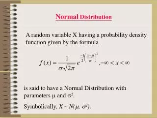
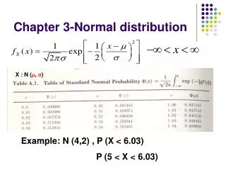
Chapter 3-Normal distribution X : N (, ) Example: N (4,2) , P (X < 6.03) P (5 < X < 6.03)
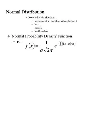
fX(x) x lognormal distribution
lognormal distribution If X ~LN (l, z) lnX ~ N (l, z)
Example • 1. F-1(0.95) = 1.645 • How about the settlement is Log-normal?
fX(x) l x exponential distribution x 0
fX(x) x Beta distribution q = 2.0 ; r = 6.0 probability b = 12 a = 2.0
Standard Beta distribution fX(x) (a = 0, b = 1) q = 1.0 ; r = 4.0 q = r = 3.0 q = 4.0 ; r = 2.0 q = r = 1.0 x The difference between Beta and other similar distribution
Review of Bernoulli sequence model • x success in n trials: binomial • time to first success: geometric • time to kth success: negative binomial
Ex 3.54 Statistics show that 20% of freshman in engineering school quit in 1 year. What is the probability that among eight students selected at random, two of them will quit after 1 year?
Think: 1. Continuous or discrete? Students cannot pass or fail “continuously” • Binomial, Geometric or Negative binomial? Bi: x success in n trials (orderless) Geo: time to first success (ordered) Neg: time to kth success (last term ordered) • p = 0.2
What is the probability of at least two of them will fail after 1 year? Use T.O.T: P (X ≥ 2) = 1 – P(X = 0) – P(X = 1)
what is the probability that among eight students selected at random, two of them will quit within 2 years? Approach 1: Bayes theorem + TOT We first consider 1st year scenario: Why not consider X = 3, 4…...8?
For 2nd year: P = P(0 student in 1st year) P(2 student in 2nd year) + P(1 student in 1st year) P(1 student in 2nd year) + P(2 student in 1st year) P(0 student in 2nd year) P = (.167)(.293) + (.335)(.367) + (.293)(.262) = .249
Approach 2: Geometric Recall geometric is “first time to success”, (1-p)t-1p Students can quit at 1st and 2nd year. i.e. t=1, t =2 When t = 2, 1st year pass is defined. P (t = 1) = 0.2 P (t =2) = (0.8)2-10.2 = 0.16 P (a student quit in 1 or 2 year) = 0.2 + 0.16 = 0.36