The Normal Distribution
The Normal Distribution. ST-L3 Objectives: To study the properties of the Normal Distribution. Learning Outcome B-4.

The Normal Distribution
E N D
Presentation Transcript
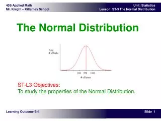
The Normal Distribution ST-L3 Objectives:To study the properties of the Normal Distribution. Learning Outcome B-4
In the first lesson, you studied central tendencies of data and also the dispersion of data. The standard deviation provided some information about how data was spread about the mean. A histogram, which is a frequency distribution graph, was used to show the spread of data.The histogram below shows the marks of all Senior 4 Applied Math students in a large school division. Note that the data are concentrated around the central part of the distribution. Note also the shape of the graph. In this lesson, you will study frequency distributions whose graphs are similar to the one shown. Theory – Intro
A Normal Distribution is a frequency distribution that can be represented by a symmetrical bell-shaped curve which shows that most of the data are concentrated around the centre (i.e., mean) of the distribution. The mean, median, and mode are all equal. Since the median is the same as the mean, 50 percent of the data are lower than the mean, and 50 percent are higher. The frequency distribution showing light bulb life (repeated below) shows that the mean is 970 hours, and the hours of life for all the bulbs are spread uniformly about the mean. Theory – The Normal Distribution
The diagram above represents a normal distribution. In real life, the data would never fit a normal distribution perfectly. There are, however, many situations where data do approximate a normal distribution. Some examples would include: • the heights and weights of adult males in North America • the times for athletes to run 5000 metres • the speed of cars on a busy highway • the weights of loonies produced at the Winnipeg Mint • Note that all the examples represent continuous data. Theory – The Normal Distribution
The data are continuous and distributed evenly around the mean, and the graph created by the data is a bell-shaped curve, as shown in the examples below. • The curve is symmetrical about the mean. Most of the data are relatively close to the mean, and the number of data decrease as you get farther from the mean. Theory – Characteristics of The Normal Distribution
3. The shape of any normal distribution curve is determined by: • the mean (m) • the standard deviation (s) • Changing the mean will shift the graph horizontally. • Changing the standard deviation will change the shape of the curve, making it narrow or wide. Theory – Characteristics of The Normal Distribution
The probability that a scorefalls within one standarddeviation of the mean isapproximately 68 percent. • The probability that a scorefalls within two standarddeviations of the mean isapproximately 95 percent. • The probability that a scorefalls within three standarddeviations of the mean isapproximately 99.7 percent. Theory – Characteristics of The Normal Distribution
The chart shows the ages in years of 30 trees in an area of natural vegetation.Determine whether the data approximate the normal distribution. • Procedure 1:Calculate the mean and standard deviation. Then determine whether approximately 68 percent of the data fall within one standard deviation of the mean.Using Winstats : • = 27.5 years, s = 8.3 years Now do the following calculations:i.e., 53 percent of the trees are within one standard deviation of the meanIn a normal distribution, this should be about 68 percent.Therefore, the data (ages of trees) do not approximate a normal distribution. Example - Do Data Approximate a Normal Distribution?
Procedure 2:Use Winstats to sketch a histogram of the data. The shape of the histogram does not approximate a normal distribution (i.e., the bell-shaped curve), and so the ages of the trees are not normally distributed. Example - Do Data Approximate a Normal Distribution?
The chart shows the sizes of pants sold in one week at Dan's Clothing Shop. Sample Problem - Do Data Approximate a Normal Distribution? (Calculations)
Sample Problem - Do Data Approximate a Normal Distribution? (Calculations)
The chart shows the sizes of pants sold in one week at Dan's Clothing Shop. Sample Problem - Do Data Approximate a Normal Distribution? (Histogram)
A machine is used to fill bags with beans. The machine is set to add 10 kilograms of beans to each bag. The table shows the weights of 277 bags that were randomly selected. • Are the weights normally distributed? How do you know? • Do you think that using the machine is acceptable and fair to the customers? Explain your reasoning. Grouped Data
Forty students measured the width of the gym, and wrote their measurements in centimetres, rounded to the nearest cm. The measurements are recorded on the table below. Use Winstats to draw a histogram of the data. Is the data approximately a normal distribution? Drawing a Histogram from Raw Data
Solution:First you need to determine the following parameters:range = 2255 - 2245 = 10 cmMin val … = 2244.5 cm (or 2245 cm) (i.e. at or just below the lowest value)Number … = 11 (i.e. 11 bars in the histogram)Width … = 0.1 (10cm/11 bars 0.1)Now draw the histogram by selecting Stats, and then Histogram. You may now select Normal to show the normal curve superimposed on the histogram.Answer:The histogram shows that thedata are approximately a normaldistribution. Drawing a Histogram from Raw Data