Demand Management and Forecasting
Demand Management and Forecasting. Chapter 15. Learning Objectives. Understand the role of forecasting as a basis for supply chain planning. Compare the differences between independent and dependent demand.

Demand Management and Forecasting
E N D
Presentation Transcript
Demand Management and Forecasting Chapter 15
Learning Objectives • Understand the role of forecasting as a basis for supply chain planning. • Compare the differences between independent and dependent demand. • Identify the basic components of independent demand: average, trend, seasonal, and random variation. • Describe the common qualitative forecasting techniques such as the Delphi method and Collaborative Forecasting. • Show how to make a time series forecast using regression, moving averages, and exponential smoothing.
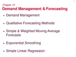
Demand Management • Strategic forecasts: forecasts used to help set the strategy of how demand will be met • Tactical forecasts: forecasted needed for how a firm operates processes on a day-to-day basis • The purpose of demand management is to coordinate and control all sources of demand • Two basic sources of demand • Dependent demand: the demand for a product or service caused by the demand for other products or services • Independent demand: the demand for a product or service that cannot be derived directly from that of other products LO 2
Independent Demand: Finished Goods Dependent Demand: Raw Materials, Component parts, Sub-assemblies, etc. A C(2) B(4) D(2) E(1) D(3) F(2) Demand Management
Components of Demand • Average demand for a period of time • Trend • Seasonal element • Cyclical elements • Random variation • Autocorrelation
Seasonal variation x Linear Trend x x x x x x x x x x x Sales x x x x x x x x x x x x x x x x x x x x x x x x x x x x x x x x x x x 1 2 3 4 Year Finding Components of Demand
Types of Forecasts • Qualitative (Judgmental) • Quantitative • Time Series Analysis • Causal Relationships • Simulation
Qualitative Methods Executive Judgment Grass Roots Qualitative Methods Market Research Historical analogy Delphi Method Panel Consensus
Delphi Method l. Choose the experts to participate. There should be a variety of knowledgeable people in different areas. 2. Through a questionnaire (or E-mail), obtain forecasts (and any premises or qualifications for the forecasts) from all participants. 3. Summarize the results and redistribute them to the participants along with appropriate new questions. 4. Summarize again, refining forecasts and conditions, and again develop new questions. 5. Repeat Step 4 if necessary. Distribute the final results to all participants.
Time Series Analysis • Time series forecasting models try to predict the future based on past data. • You can pick models based on: 1. Time horizon to forecast 2. Data availability 3. Accuracy required 4. Size of forecasting budget 5. Availability of qualified personnel
Time Series Analysis • Short term: forecast under three months • Tactical decisions • Medium term: three months to two years • Capturing seasonal effects • Long term: forecast longer than two years • Detecting general trends • Identifying major turning points LO 5
Simple Moving Average Formula • The simple moving average model assumes an average is a good estimator of future behavior. • The formula for the simple moving average is: Ft = Forecast for the coming period N = Number of periods to be averaged A t-1 = Actual occurrence in the past period for up to “n” periods
Simple Moving Average Problem (1) • Question: What are the 3-week and 6-week moving average forecasts for demand? • Assume you only have 3 weeks and 6 weeks of actual demand data for the respective forecasts
14 Calculating the moving averages gives us: F4=(650+678+720)/3 =682.67 F7=(650+678+720 +785+859+920)/6 =768.67 • The McGraw-Hill Companies, Inc., 2001
Weighted Moving Average Formula While the moving average formula implies an equal weight being placed on each value that is being averaged, the weighted moving average permits an unequal weighting on prior time periods. The formula for the moving average is: wt = weight given to time period “t” occurrence. (Weights must add to one.)
Choosing Weights • Experience and trial-and-error are the simplest ways • Generally, the most recent past is the best indicator • When data are seasonal, weights should be established accordingly LO 5
Weighted Moving Average Problem (1) Data Question: Given the weekly demand and weights, what is the forecast for the 4th period or Week 4? Weights: t-1 .5 t-2 .3 t-3 .2 Note that the weights place more emphasis on the most recent data, that is time period “t-1”.
Weighted Moving Average Problem (1) Solution F4 = 0.5(720)+0.3(678)+0.2(650)=693.4
Exponential Smoothing • Most used of all forecasting techniques • Integral part of all computerized forecasting programs • Widely used in retail and service • Widely accepted because… • Exponential models are surprisingly accurate • Formulating an exponential model is relatively easy • The user can understand how the model works • Little computation is required to use the model • Computer storage requirements are small • Tests for accuracy are easy to compute LO 5
Exponential Smoothing Model • Premise: The most recent observations might have the highest predictive value. • Therefore, we should give more weight to the more recent time periods when forecasting. Ft = Ft-1 + a(At-1 - Ft-1) a = smoothing constant
Exponential Smoothing Problem (1) Data • Question: Given the weekly demand data, what are the exponential smoothing forecasts for periods 2-10 using a=0.10 and a=0.60? • Assume F1=D1
Answer: The respective alphas columns denote the forecast values. Note that you can only forecast one time period into the future.
Exponential Smoothing Problem (1) Plotting Note how that the smaller alpha the smoother the line in this example.
Simple Linear Regression Model Y The simple linear regression model seeks to fit a line through various data over time. a 0 1 2 3 4 5 x (Time) Yt = a + bx Is the linear regression model. Yt is the regressed forecast value or dependent variable in the model, a is the intercept value of the the regression line, and b is similar to the slope of the regression line. However, since it is calculated with the variability of the data in mind, its formulation is not as straight forward as our usual notion of slope.
Simple Linear Regression Formulas for Calculating “a” and “b”
Simple Linear Regression Problem Data Question: Given the data below, what is the simple linear regression model that can be used to predict sales?
Answer: First, using the linear regression formulas, we can compute “a” and “b”. 27 • The McGraw-Hill Companies, Inc., 2001
The resulting regression model is: Yt = 143.5 + 6.3x 28 Now if we plot the regression generated forecasts against the actual sales we obtain the following chart: 180 175 170 165 Sales 160 155 Forecast Sales 150 145 140 135 1 2 3 4 5 Period • The McGraw-Hill Companies, Inc., 2001
Forecast Error • Bias errors: when a consistent mistake is made • Random errors: errors that cannot be explained by the forecast model being used • Measures of error • Mean absolute deviation (MAD) • Mean absolute percent error (MAPE) • Tracking signal LO 5
The MAD Statistic to Determine Forecasting Error • The ideal MAD is zero. That would mean there is no forecasting error. • The larger the MAD, the less the desirable the resulting model.
Month Sales Forecast 1 220 n/a 2 250 255 3 210 205 4 300 320 5 325 315 MAD Problem Data Question: What is the MAD value given the forecast values in the table below?
Month Sales Forecast Abs Error 1 220 n/a 2 250 255 5 3 210 205 5 4 300 320 20 5 325 315 10 40 MAD Problem Solution Note that by itself, the MAD only lets us know the mean error in a set of forecasts.
Tracking Signal Formula • The TS is a measure that indicates whether the forecast average is keeping pace with any genuine upward or downward changes in demand. • Depending on the number of MAD’s selected, the TS can be used like a quality control chart indicating when the model is generating too much error in its forecasts. • The TS formula is: