Demand Management and Forecasting
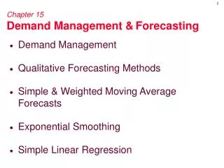
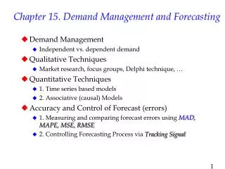
Demand Management and Forecasting. Chapter 15. 15- 2. OBJECTIVES. Focus on two short-range forecasting techniques Moving Average Exponential Smoothing. 15- 3. Simple Moving Average Formula. The simple moving average model assumes an average is a good estimator of future behavior

Demand Management and Forecasting
E N D
Presentation Transcript
Demand ManagementandForecasting Chapter 15
15-2 OBJECTIVES Focus on two short-range forecasting techniques • Moving Average • Exponential Smoothing
15-3 Simple Moving Average Formula • The simple moving average model assumes an average is a good estimator of future behavior • The formula for the simple moving average is: Ft = Forecast for the coming period N = Number of periods to be averaged A t-1 = Actual occurrence in the past period for up to “n” periods
15-4 Simple Moving Average Problem (1) Question: What are the 3-week and 6-week moving average forecasts for demand? Assume you only have 3 weeks and 6 weeks of actual demand data for the respective forecasts
15-5 F4=(650+678+720)/3 =682.67 F7=(650+678+720 +785+859+920)/6 =768.67 Calculating the moving averages gives us: • The McGraw-Hill Companies, Inc., 2004
15-6 Plotting the moving averages and comparing them shows how the lines smooth out to reveal the overall upward trend in this example Note how the 3-Week is smoother than the Demand, and 6-Week is even smoother
15-7 Simple Moving Average Problem (2) Data Question: What is the 3 week moving average forecast for this data? Assume you only have 3 weeks and 5 weeks of actual demand data for the respective forecasts
15-8 F4=(820+775+680)/3 =758.33 F6=(820+775+680 +655+620)/5 =710.00 Simple Moving Average Problem (2) Solution
15-9 Exponential Smoothing Model Ft = Ft-1 + a(At-1 - Ft-1) • Premise: The most recent observations might have the highest predictive value • Therefore, we should give more weight to the more recent time periods when forecasting
15-10 Exponential Smoothing Problem (1) Data Question: Given the weekly demand data, what are the exponential smoothing forecasts for periods 2-10 using a=0.10 and a=0.60? Assume F1=D1
15-11 Answer: The respective alphas columns denote the forecast values. Note that you can only forecast one time period into the future.
15-12 Exponential Smoothing Problem (1) Plotting Note how that the smaller alpha results in a smoother line in this example
15-13 Exponential Smoothing Problem (2) Data Question: What are the exponential smoothing forecasts for periods 2-5 using a =0.5? Assume F1=D1
15-14 F1=820+(0.5)(820-820)=820 Exponential Smoothing Problem (2) Solution F3=820+(0.5)(775-820)=797.75
15-15 The MAD Statistic to Determine Forecasting Error • The ideal MAD is zero which would mean there is no forecasting error • The larger the MAD, the less the accurate the resulting model
15-16 MAD Problem Data Question: What is the MAD value given the forecast values in the table below? Month Sales Forecast 1 220 n/a 2 250 255 3 210 205 4 300 320 5 325 315
15-17 Month Sales Forecast Abs Error 1 220 n/a 2 250 255 5 3 210 205 5 4 300 320 20 5 325 315 10 40 MAD Problem Solution Note that by itself, the MAD only lets us know the mean error in a set of forecasts
MAPE • Mean Absolute Percentage Error (MAPE) is another measure often used to evaluate forecasting accuracy A MAPE of under 8% is acceptable for most applications
15-20 Question Bowl Which of the following is an example of a “Time Series Analysis” type of forecasting technique or model? • Simulation • Exponential smoothing • Panel consensus • All of the above • None of the above Answer: b. Exponential smoothing (Also includes Simple Moving Average, Weighted Moving Average, Regression Analysis, Box Jenkins, Shiskin Time Series, and Trend Projections.)
15-21 Question Bowl Which of the following are reasons why the Exponential Smoothing model has been a well accepted forecasting methodology? • It is accurate • It is easy to use • Computer storage requirements are small • All of the above • None of the above Answer: d. All of the above
15-22 Question Bowl The value for alpha or α must be between which of the following when used in an Exponential Smoothing model? • 1 to 10 • 1 to 2 • 0 to 1 • -1 to 1 • Any number at all Answer: c. 0 to 1
15-23 Question Bowl Which of the following are sources of error in forecasts? • Bias • Random • Employing the wrong trend line • All of the above • None of the above Answer: d. All of the above
15-24 Question Bowl Which of the following would be the “best” MAD values in an analysis of the accuracy of a forecasting model? • 1000 • 100 • 10 • 1 • 0 Answer: e. 0
15-25 End of Chapter 15