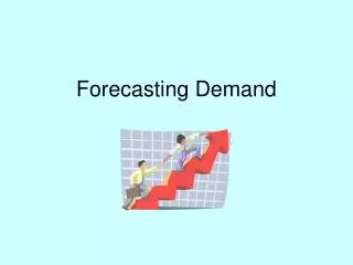
Forecasting Demand
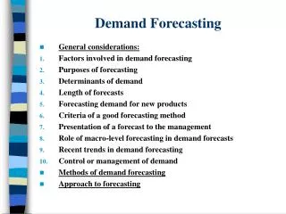
Forecasting Demand. Chapter 11. Forecasting Demand. Subjective Models Delphi Method Cross-Impact Historical Analogy Causal Models Regression Models Econometric Models Time Series Models N-Period Moving Average Simple Exponential Smoothing

Forecasting Demand
E N D
Presentation Transcript
Forecasting Demand Chapter 11
Forecasting Demand • Subjective Models • Delphi Method • Cross-Impact • Historical Analogy • Causal Models • Regression Models • Econometric Models • Time Series Models • N-Period Moving Average • Simple Exponential Smoothing • Exponential Smoothing with Trend or Seasonal Adjustment
Subjective Models • Delphi Method • Developed at the Rand Corporation by Olaf Helmer • Method is based on expert opinion • People with expertise are asked to answer some question (no interaction among respondents) • Answers are grouped and the placed into quartiles based on the frequency in which they were mentioned • Respondents review the results and answers in the extreme quartiles must be justified. • Continued iterative process
Subjective Models • Cross-Impact Analysis • This analysis assumes that a future event is related to the occurrence of an earlier event • If historical data shows that as gas prices go up by 50 cents a gallon, mass transit rider-ship increases by 100 people • If there are deviations in this trend, experts go back and evaluate what happened
Subjective Models • Historical Analogy • Assumes the introduction and growth pattern of a new service will mimic the pattern of a similar concept
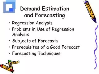
Causal Models • Regression Analysis • Shows the relationship between a dependent variable and one or more independent variables • Independent Variables: Age, IQ • Dependent Variable: Computer Ability • To what extent do age and IQ impact computer ability?
Causal Models • Econometrics • Similar to regression models • Involves a system of equations that are related to each other • Solve for simultaneous equations that express the dependent variable in terms of several different independent variables
Time Series Models • N Period Moving Average • This approach smoothes out random fluctuations that may occur • As a manager, you don’t want to overreact to random changes • MAT = (AT + AT-1 + AT-2 + …..+ AT-N+1)/N • where: MAT = The N period moving average • AT = Actual observation for period T
3 Period Moving Average Example Saturday Occupancy at a 100-room Hotel Three-period Saturday Period Occupancy Moving Average Forecast Aug. 1 1 79 8 2 84 15 3 83 82* 22 4 81 83** 82 29 5 98 87 83 Sept. 5 6 100 93 87 12 7 93 * (83+84+79)/3 = 82 ** (84+83+81)/3 = 82.67 ≈ 83
N Period Moving Average • Very inexpensive and easy to understand • Gives equal weight to all observations • Does not consider observations older than N periods
Time Series Models Simple Exponential Smoothing • Most frequently used for demand forecasting • Based on the concept of feeding back the “forecast error” to correct the previous smoothed value St = St-1 + α (At – St-1) Where: St = smoothed value for time period t (At – St-1) represents the forecast error α = a weight which allows the manager to determine how much weight or importance to give to recent data (large values give higher values to recent data)
Simple Exponential Smoothing Example Saturday Hotel Occupancy ( α=0.5) Actual Smoothed Forecast Period Occupancy Value Forecast Error Saturday t At St Ft |At - Ft| Aug. 1 1 79 79.00 8 2 84 81.50* 79 5# 15 3 83 82.25** 82 1 22 4 81 82.88 82 1 29 5 98 90.44 83 15 Sept. 5 6 100 95.22 90 10 *79.00 + 0.5 (84.00 - 79.00) = 81.50 ** 81.50 + 0.5 (83.00 - 81.50) = 82.25 # 84.00 – 79.00 = 5
Simple Exponential Smoothing • This approach helps to prevent over-reaction to extremes in observed values • The older observations never disappear entirely from the calculation of St like they do in N Period Moving Average approach • To measure the accuracy of our forecasts, we can calculate the Mean Absolute Deviation (MAD)
Simple Exponential Smoothing Example Saturday Hotel Occupancy ( α=0.5) Actual Smoothed Forecast Period Occupancy Value Forecast Error Saturday t At St Ft |At - Ft| Aug. 1 1 79 79.00 8 2 84 81.50* 79 5# 15 3 83 82.25** 82 1 22 4 81 82.88 82 1 29 5 98 90.44 83 15 Sept. 5 6 100 95.22 90 10 MAD = 6.4 MAD = (5 + 1 + 1 + 15 + 10) / 5 *79.00 + 0.5 (84.00 - 79.00) = 81.50 ** 81.50 + 0.5 (83.00 - 81.50) = 82.25 # 84.00 – 79.00 = 5
Exponential Smoothing with Trend Adjustment • A trend in a set of Data is the average rate at which the observed values change from one period to the next over time. • Requires the addition of the trend value to the smoothed value equation • St = α(At) + (1- α) (St-1 + Tt-1) • Tt = β (St – St-1) + (1 – β) Tt-1 • Ft+1 = St + Tt