
Threshold Liability Models (Ordinal Data Analysis)
E N D
Presentation Transcript
Threshold Liability Models(Ordinal Data Analysis) Frühling Rijsdijk MRC SGDP Centre, Institute of Psychiatry, King’s College London Boulder Twin Workshop 2014
Ordinal data • Measuring instrument discriminates between two or a few ordered categories e.g.: • Absence (0) or presence (1) of a disorder • Score on a single Q item e.g. : 0 - 1, 0 - 4 • In such cases the data take the form of counts, i.e. the number of individuals within each category of response
Analysis of ordinal variables • The session aims to show how we can estimate correlations from simple count data (with the ultimate goal to estimate h2, c2, e2) • For this we need to introduce the concept of ‘Liability’ or ‘liability threshold models’ • This is followed by a more mathematical description of the model • Practical session
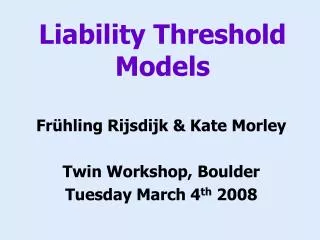
Liability • Liability is a theoretical construct. It’s the underlying continuous variable of a variable which we were only able to measure in terms of a few ordered categories • Assumptions: • Standard Normal Distribution (2) 1 or more thresholds (cut-offs) to discriminate between the ordered response categories
68% -2 3 - 0 1 1 2 -3 The Standard Normal Distribution Standard Normal Distribution (SND) or z-distribution: • Mathematically described by the SN Probability Density function ( =phi), a bell-shaped curve with: • mean (µ)= 0 and SD (σ) = 1 • z-values are the number of SD away from the mean • Convenience: area under curve =1, translates directly to probabilities
P(Tc≤ y ≤ Tc+1) TC+1 3 -3 0 Standard Normal Cumulative Probability function • Observed ordinal measure (Y) with C categories is related to the underlying continuous variable (y) by means of C-1 thresholds (Tc) • Probability that yis in category c (i.e., the probability that y is between the two thresholds) is the area under the standard normal curve bounded by the two thresholds on the z scale (Tc & Tc+1) 1 2 0 TC
Area under the curve • Mathematically, the area under a curve can be worked out using integral calculus. This is the mathematical notation for the area between the thresholds (category 1):
Area under the curve • Category 0: The area between –infinity and threshold Tc: • Category 2: The area between threshold Tc+1 and +infinity
Ordinal trait measured in twin pairs: 2 categories (1 Threshold) Contingency Table with 4 observed cell counts representing the number of pairs for all possible response combinations a = 00 e = 11 b = 01 d = 10
Joint Liability r =.90 r =.00
The observed cell proportions relate to the proportions of the BND with a certain correlation between the latent variables (y1 and y2), each cut at a certain threshold • i.e. the joint probability of a certain response combination is the volume under the BND surface bounded by appropriate thresholds on each liability
Expected cell proportions Numerical integration of the BND over the two liabilities e.g. the probability that both twins are above Tc : Φis the bivariate normal probability density function, y1andy2 are the liabilities of twin1 and twin2, with means of0,and the correlation between the two liabilities Tc1is threshold (z-value) ony1,Tc2is threshold (z-value) ony2
Estimation of Correlations and Thresholds • Since the BN distribution is a known mathematical distribution, for each correlation (∑) and any set of thresholds on the liabilities we know what the expected proportions are in each cell. • Therefore, observed cell proportions of our data will inform on the most likely correlation and threshold on each liability. r = 0.60 Tc1=Tc2 = 1.4 (z-value)
Bivariate Ordinal Likelihood • The likelihood for each observed ordinal response pattern is computed by the expected proportion in the corresponding cell of the BN distribution • The maximum-likelihood equation for the whole sample is -2* log of of the likelihood of each vector of observation, and summing across all observations (pairs) • This -2LL is minimized to obtain the maximum likelihood estimates of the correlation and thresholds • Tetra-choric correlation if y1 and y2 reflect 2 categories (1 Threshold); Poly-choric when >2 categories per liability
Twin Models • Estimate correlation in liabilities separately for MZ and DZ pairs from their Count data • Variance decomposition (A, C, E) can be applied to the underlying latent variable or liability of the trait • Estimate of the heritability of the liability
Variance constraint Threshold model ACE Liability Model 1 1/.5 E C A A C E L L 1 1 Af Unaf Unaf Af Twin 1 Twin 2
Summary • OpenMx models ordinal data under a threshold model • Assumptions about the (joint) distribution of the data (Standard Bivariate Normal) • The relative proportions of observations in the cells of the Contingency Table are translated into proportions under the SBN • The most likely thresholds and correlations are estimated • Genetic/Environmental variance components are estimated based on these correlations derived from MZ and DZ data
Test of BN assumption For a 2x2 CT with 1 estimated TH on each liability, the 2 statistic is always zero, i.e. with 3 observed statistics, estimating 3 parameters, DF=0 (it is always possible to find a correlation and 2 TH to perfectly explain the proportions in each cell). No goodness of fit of thenormal distribution assumption. This problem is resolved if the CT is at least 2x3 (i.e. more than 2 categories on at least one liability) A significant 2 reflects departure from normality.
Power issues • Ordinal data / Liability Threshold Model: less power than analyses on continuous data Neale, Eaves & Kendler 1994 • Solutions: 1. Bigger samples 2. Use more categories controls controls cases cases sub-clinical
Practical Example R Script: ThresholdLiab.R Data File: CASTage8.csv
Sample & Measures • CAST data collected at age 8 in the TEDS sample • Parent report of CAST: Childhood Asperger Syndrome Test (Scott et al., 2002) • Includes children with autism spectrum disorder • Twin pairs: 501 MZ & 503 DZ males
Clinical Aspects of the CAST The CAST score dichotomized at around 96% (i.e. scores of >15), is the clinical cut-off point for children at risk for Autism Spectrum Disorder However, for the purpose of this exercise, we will use 2 cut offs to create 3 categories: <9 un-affacted (0) 9-15 sub-clinical (1) >15 ASD (2)
Inspection of the data CAST score categorized (0,1,2), the proportions: Ccast | Freq. Percent ------------+-------------------------- 0 | 804 80.08 1 | 158 15.74 2 | 42 4.18 ------------+--------------------------- Total | 1,004 100.00 Z-values 20% 4% 3 -3 .84 1.75 Z-value Th1 = .84 Z-value Th2 = 1.75
How to find Z-values • Standard Normal Cumulative Probability Tables • Excel • =NORMSINV() 8% 92% 3 -3 0 -1.4 1.4
CTs of the MZ and DZ pairs table(mzData$OFcast1, mzData$OFcast2 ) table(dzData$OFcast1, dzData$OFcast2 )
R Script: ThresholdLiab.R Castdata <- read.table ('CASTage8.csv', header=T, sep=‘,’, na.strings=".") # Make the integer variables ordered factors Castdata$OFcast1 <-mxFactor(Castdata$Ccast1, levels=c(0:2) ) Castdata$OFcast2 <-mxFactor(Castdata$Ccast2, levels=c(0:2) ) selVars <-c('OFcast1' , 'OFcast2') useVars <-c('OFcast1' , 'OFcast2', 'age1', 'age2') # Select Data for Analysis mzData <- subset(Castdata, zyg==1, useVars) dzData <- subset(Castdata, zyg==2, useVars) Ordinal variables MUST be specified as ordered factors in the included data. The function prepares ordinal variables as ordered factors in preparation for inclusion in OpenMx models. Factors contain a ‘levels’ argument.
# Matrices for expected Means (SND) & correlations mean <-mxMatrix( type="Zero", nrow=1, ncol=ntv, name="M" ) corMZ <-mxMatrix(type="Stand", nrow=ntv, ncol=ntv, free=T, values=.6, lbound=-.99, ubound=.99, name="expCorMZ") CorDZ <-mxMatrix(type="Stand", nrow=ntv, ncol=ntv, free=T, values=.3, lbound=-.99, ubound=.99, name="expCorDZ") 0,0 1 1 r L1 L2 L1 L2 L1 L2 1 1 rMZ rDZ 1 1 L1 L1 1 1 C1 C2 rDZ rMZ L2 L2
The Threshold model Twin 2 Twin 2 Twin 1 Twin 1 Tmz11Tmz21 Tmz12Tmz22 Tdz11Tdz21 Tdz12Tdz22 Tmz11 Tdz11 Tmz21 Tdz21 Tmz22 Tmz12 Tdz22 Tdz12
Specification imz11 imz12 idz11 idz12 Twin 1 Twin 1 Twin 2 Twin 2 Tmz12 Tdz11 Tdz12 Tmz11 Tdz21=Tdz11+idz11 Tmz22=Tmz12+imz12 Tdz22=Tdz12+idz12 Tmz21=Tmz11+imz11
A multiplication is used to ensure that any threshold is higher than the previous one. This is necessary for the optimization procedure involving numerical integration over the MVN Expected Thresholds: L %*% ThMZ="expThreMZ" 1 0 1 1 TMZ11TMZ12 iMZ11iMZ12 TMZ11TMZ12 TMZ11+iMZ11TMZ12+ iMZ12 = * expThmz Threshold 1 for twin 1 and twin2 TMZ11TMZ12 TMZ21 TMZ22 Threshold 2 for twin 1 and twin2 Note: this only works if the increments are POSITIVE values, therefore a BOUND statement around the increments are necessary
Start Values & Bounds # nth max number of thresholds; ntv number of variables per pair Tmz <-mxMatrix(type="Full", nrow=nth, ncol=ntv, free=TRUE, values=c(.8, 1), lbound=c(-3, .001 ), ubound=3, labels=c("Tmz11","imz11", "Tmz12","imz12"), name="ThMZ") TMZ11TMZ12 iMZ11 iMZ12 .8 (-3-3).8 (-3- 3) 1(.001 -3)1(.001-3) = The positive bounds on the increments stop the thresholds going ‘backwards’, i.e. they preserve the ordering of the categories Z-value Th1 = .84 Z-value Th2 = 1.75
Threshold model: add effect of AGE # Specify matrices to hold the definition variables (covariates) and their effects obsAge <- mxMatrix( type="Full", nrow=1, ncol=2, free=F, labels=c("data.age1","data.age2"), name="Age") betaA <-mxMatrix( type="Full", nrow=nth, ncol=1, free=T, values=c(-.2), labels=c('BaTH'), name="BageTH" ) ThresMZ <-mxAlgebra( expression= L%*%ThMZ + BageTH %x% Age, name = expThresMZ ) ‘BageTH’ BaTH BaTH = %x% age1 age2 ‘Age’: definition variables Effect of age on Th1 tw1 Effect of age on Th1 tw2 Effect of age on Th2 tw1Effect of age on Th2 tw2
# Objective objects for Multiple Groups objMZ <- mxFIMLObjective( covariance="expCorMZ", means="M", dimnames=selVars, thresholds="expThresMZ" ) objDZ <- mxFIMLObjective( covariance="expCorDZ", means="M", dimnames=selVars, thresholds="expThresDZ" ) Objective functions are functions for which free parameter values are chosen such that the value of the objective function is minimized mxFIMLObjective: Objective functions which uses Full–Information maximum likelihood, the preferred method for raw data
# Objective objects for Multiple Groups objMZ <- mxFIMLObjective( covariance="expCorMZ", means="M", dimnames=selVars, thresholds="expThresMZ" ) objDZ <- mxFIMLObjective( covariance="expCorDZ", means="M", dimnames=selVars, thresholds="expThresDZ" ) Ordinal data requires an additional argument for the thresholds Also required is ‘dimnames’ (dimension names) which corresponds to the ordered factors you wish to analyze, defined in this case by ‘selVars’
# RUN SUBMODELS # SubModel 1: Thresholds across Twins within zyg group are equal Sub1Model <- mxModel(SatModel, name=“sub1”) Sub1Model <- omxSetParameters( Sub1Model, labels=c("Tmz11", “imz11", "Tmz12", “imz12"), newlabels=c("Tmz11", “imz11", "Tmz11", “imz11"), … # SubModel 2: Thresholds across Twins & zyg group Sub2Model <- mxModel(SatModel, name="sub2") Sub2Model <- omxSetParameters(Sub2Model, labels=c("Tmz11",“imz11","Tmz12",“imz12"), newlabels=c("Tmz11",“imz11","Tmz11",“imz11"), .... Sub2Model <- omxSetParameters(Sub2Model, labels=c("Tdz11",“idz11","Tdz12",“idz12"), newlabels=c("Tmz11",“imz11","Tmz11",“imz11"), .... omxSetParameters: function to modify the attributes of parameters in a model without having to re-specify the model
# ACE MODEL # Matrices to store a, c, and e Path Coefficients pathA <- mxMatrix( type=“Lower", nrow=nv, ncol=nv, free=TRUE, values=.6, label="a11", name="a" ) pathC <- mxMatrix( type=“Lower", nrow=nv, ncol=nv, free=TRUE, values=.6, label="c11", name="c" ) pathE <- mxMatrix( type=“Lower", nrow=nv, ncol=nv, free=TRUE, values=.6, label="e11", name="e" ) # Algebra for Matrices to hold A, C, and E Variance Components covA <- mxAlgebra( expression=a %*% t(a), name="A" ) covC <- mxAlgebra( expression=c %*% t(c), name="C" ) covE <- mxAlgebra( expression=e %*% t(e), name="E" ) covP <- mxAlgebra( expression=A+C+E, name="V" ) # Constrain Total variance of the liability to 1 matUnv <-mxMatrix( type="Unit", nrow=nv, ncol=1, name="Unv" ) varL <-mxConstraint( expression=diag2vec(V)==Unv, name="VarL" ) E C A L 1 A + C + E 1
Part (1) • Run script up to ‘Descriptive Statistics’ and check that the MZ and DZ Contingency tables are the same as in the slides • Run script up to sub2Model and check that you get the same answers as in the results slide • What are the conclusions about the thresholds, i.e. what is the final model? • What kind of Genetic model would you run on this data given the correlations? R Script: ThresholdLiab.R Data File: CASTage8.csv
Part (2) • Run the Genetic model and check that you get the same estimates (with 95% CI) as in the results slide • Exercise: Add sub-model AE at the end of the ACE model to test significance of C. For an example, see code in Hermine’s ACE script.
1 Thresh/inc: MZ tw1 = 1.85, .84 MZ tw2 = 1.7, .73 DZ tw1 = 1.67, .91 DZ tw2 = 1.75, .72 2 Thresh/inc: MZ = 1.90, .78 DZ = 1.74, .81 3 Thresh/inc: 1.81, .80 The Twin correlations for model 3 are: rMZM = 0.82 (.74 - .87) rDM = 0.43 (.29 - .56) BetaAge: -.12 (-.18 / .02)
ACE Estimates for the ordinalized CAST score in Boys at age 8 Name ep -2LL df AIC Model 1 : ACE 6 2208.2 2004 -1799.84
More Scripts • Univariate Ordinal example with estimated Means and Variances (CAST variable with 3 categories) • Script: UnivM&Sdord.R(This topic will be covered tomorrow by Sarah in tomorrows extra morning session) • Bivariate Ordinal example with unequal thresholds (IQ, 2 categories, ADHD, 3 categories) • Script: BivThreshLiab23.R • Bivariate combined Continuous-Ordinal example (IQ, continuous, ADHD, 3 categories) • Script: BivOrdCont.R(This topic will be covered tomorrow afternoon)