Wind Driven Circulation III
This article explores the vorticity equation in physical oceanography and its relevance to wind-driven circulation. It covers concepts such as closed gyre circulation, quasi-geostrophic vorticity equation, westward intensification, Stommel model, Munk model, inertia boundary layer, numerical results, and observations. The text is in English.


Wind Driven Circulation III
E N D
Presentation Transcript
Wind Driven Circulation III • Closed Gyre Circulation • Quasi-Geostrophic Vorticity Equation • Westward intensification • Stommel Model • Munk Model • Inertia boundary layer • Numerical results • Observations
Vorticity Equation In physical oceanography, we deal mostly with the vertical component of vorticity , which is notated as From horizontal momentum equation, (1) (2) Taking , we have
For a rotating solid object, the vorticity is two times of its angular velocity
Considering the case of constant ρ. For a shallow layer of water (depth H<<L), u and v are not function of z because the horizontal pressure gradient is not a function of z. (In general, the vortex tilting term, is usually small. Then we have the simplified vorticity equation Since the vorticity equation can be written as (ignoring friction) ζ+f is the absolute vorticity
Using the Continuity Equation For a layer of thickness H, consider a material column We get or Potential Vorticity Equation
Alternative derivation of Sverdrup Relation Construct vorticity equation from geostrophic balance (1) (2) Integrating over the whole ocean depth, we have is the entrainment rate from the Ekman layer where at 45oN The Sverdrup transport is the total of geostrophic and Ekman transport. The indirectly driven Vg may be much larger than VE.
In the ocean’s interior, for large-scale movement, we have the differential form of the Sverdrup relation i.e., ζ<<f
A more general form of the Sverdrup relation Ekman layer at bottom Spatially changing sea surface height η and bottom topography zB and pressure pB. Assume atmospheric pressure pη≈0. Let , Integrating over the vertical column, we have Similarly
Define Ep is the work done to pile up the water above the bottom is the total potential energy of sea water with S=35, T=0oC function of bottom topography only is the potential energy anomaly
It can be shown that Therefore, the balance of forces can be written as
Define Baroclinic geostrophic transport Barotropic geostrophic transport Ekman transport in the surface layer Ekman transport in the bottom layer Therefore, we have
Following Sverdrup’s approach, we take Surface stress curl Bottom stress curl Bottom topography effect Vanish if the bottom is flat Or flow follows topographic contour Net baroclinic geostrophic transport is zero