Download
1 / 61
610 likes | 656 Vues
Explore the fundamentals of digital and analog communication systems, including sources, waveforms, channel capacity, and ideal communication systems. Learn about measuring information, channel capacity optimization, signal properties, and physically realizable waveforms in this comprehensive lecture.

E N D
x(t) t x(t) t Analog Digital Digital and Analog Sources and Systems Basic Definitions: • Analog Information Source: An analog information source produces messages which are defined on a continuum. (E.g. :Microphone) • Digital Information Source: A digital information source produces a finite set of possible messages. (E.g. :Typewriter)
Digital and Analog Sources and Systems • A digital communication systemtransfers information from a digital source to the intended receiver (also called the sink). • An analog communication systemtransfers information from an analog source to the sink. • Adigital waveformis defined as a function of time that can have a discrete set of amplitude values. • An Analog waveformis a function that has a continuous range of values.
Deterministic and Random Waveforms • ADeterministic waveformcan be modeled as a completely specified function of time. • ARandom Waveform(or stochastic waveform) cannot be modeled as a completely specified function of time and must be modeled probabilistically. • We will focus mainly on deterministic waveforms.
Receiver Transmitter Block Diagram of A Communication System • All communication systems contain three main sub systems: • Transmitter • Channel • Receiver
Measuring Information • Definition:Information Measure (Ij) The information sent from a digital source (Ij) when the jth massage is transmitted is given by: where Pjis the probability of transmitting the jth message. • Messages that are less likely to occur (smaller value for Pj) provide more information (large value of Ij). • The information measure depends on only the likelihood of sending the message and does not depend on possible interpretation of the content. • For units of bits, the base 2 logarithm is used; • if natural logarithm is used, the units are “nats”; • if the base 10 logarithm is used, the units are “hartley”.
Measuring Information • Definition: Average Information(H) The average information measure of a digital source is, • where m is the number of possible different source messages. • The average information is also called Entropy. • Definition: Source Rate (R) The source rate is defined as, • where H is the average information • T is the time required to send a message.
Channel Capacity & Ideal Comm. Systems • For digital communication systems, the “Optimum System” may be defined as the system that minimize the probability of bit error at the system output subject to constraints on the energy and channel bandwidth. • Is it possible to invent a system with no error at the output even when we have noise introduced into the channel? • Yes under certain assumptions !. • According Shannon the probability of error would approach zero, if R< C Where • R - Rate of information (bits/s) • C - Channel capacity (bits/s) • B - Channel bandwidth in Hz and • S/N - the signal-to-noise power ratio Capacity is the maximum amount of information that a particular channel can transmit. It is a theoretical upper limit. The limit can be approached by using Error Correction
Channel Capacity & Ideal Comm. Systems ANALOG COMMUNICATION SYSTEMS In analog systems, the OPTIMUM SYSTEM might be defined as the one that achieves the Largest signal-to-noise ratio at the receiver output, subject to design constraints such as channel bandwidth and transmitted power. DIMENSIONALITY THEOREM for Digital Signalling: Nyquist showed that if a pulse represents one bit of data, noninterfering pulses can be sent over a channel no faster than 2B pulses/s, where B is the channel bandwidth.
Properties of Signals & Noise • In communication systems, the received waveform is usually categorized into two parts: • Signal: • The desired part containing the information. • Noise: • The undesired part • Properties of waveforms include: • DC value, • Root-mean-square (rms) value, • Normalized power, • Magnitude spectrum, • Phase spectrum, • Power spectral density, • Bandwidth • ………………..
Physically Realizable Waveforms • Physically realizable waveforms are practical waveforms which can be measured in a laboratory. • These waveforms satisfy the following conditions • The waveform has significant nonzero values over a composite time interval that is finite. • The spectrum of the waveform has significant values over a composite frequency interval that is finite • The waveform is a continuous function of time • The waveform has a finite peak value • The waveform has only real values. That is, at any time, it cannot have a complex value a+jb, where b is nonzero.
Physically Realizable Waveforms • Mathematical Models that violate some or all of the conditions listed above are often used. • One main reason is to simplify the mathematical analysis. • If we are careful with the mathematical model, the correct result can be obtained when the answer is properly interpreted. Physical Waveform Mathematical Model Waveform • The Math model in this example violates the following rules: • Continuity • Finite duration
Time Average Operator • Definition: The time average operatoris given by, • The operator is a linearoperator, • the average of the sum of two quantities is the same as the sum of their averages:
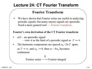
Periodic Waveforms • Definition A waveform w(t)is periodicwith period T0if, w(t) = w(t + T0)for all t where T0 is the smallest positive number that satisfies this relationship • A sinusoidal waveform of frequency f0 = 1/T0 Hertz is periodic • Theorem: If the waveform involved is periodic, the time average operator can be reduced to where T0 is the period of the waveform and a is an arbitrary real constant, which may be taken to be zero.
DC Value • Definition: The DC(direct “current”) value of a waveform w(t) is given by its time average, w(t). Thus, • For a physical waveform, we are actually interested in evaluating the DC value only over a finite interval of interest, say, from t1to t2, so that the dc value is
Decibel • A base 10 logarithmic measure of power ratios. • The ratio of the power level at the output of a circuit compared with that at the input is often specified by the decibel gain instead of the actual ratio. • Decibel measure can be defined in 3 ways • Decibel Gain • Decibel signal-to-noise ratio • Mill watt Decibel or dBm • Definition:Decibel Gain of a circuit is:
Decibel Gain • If resistive loads are involved, • Definition of dB may be reduced to, or
Fourier Transform of a Waveform • Definition: Fourier transform The Fourier Transform(FT) of a waveform w(t)is: • where ℑ[.] denotes the Fourier transform of [.] • f is the frequency parameter with units of Hz (1/s). • W(f) is also called Two-sided Spectrum of w(t), since both positive and negative frequency components are obtained from the definition
Fourier Transform of a Waveform • Definition: Inverse Fourier transform The Inverse Fourier transform(FT) of a waveform w(t) is: • The functions w(t) and W(f)constitute a Fourier transform pair. Frequency Domain Description (FT) Time Domain Description (Inverse FT)
Properties of Fourier Transforms • Theorem : Spectral symmetry of real signals If w(t) is real, then Superscript asterisk is conjugate operation. • Proof: Take the conjugate Substitute -f = • Since w(t) is real, w*(t) = w(t), and it follows that W(-f) = W*(f). • If w(t) is real and is an even function of t, W(f) is real. • If w(t) is real and is an odd function of t, W(f) is imaginary.
Corollaries of Properties of Fourier Transforms • Spectral symmetry of real signals. If w(t) is real, then: • Magnitude spectrum is even about the origin. • |W(-f)| = |W(f)| (A) • Phase spectrum is odd about the origin. • θ(-f) = - θ(f)(B) Since, W(-f) = W*(f) We see that corollaries (A) and (B) are true.
Properties of Fourier Transform • f, called frequency and having units of hertz, is just a parameter of the FT that specifies what frequency we are interested in looking for in the waveform w(t). • The FT looks for the frequency f in the w(t)over all time, that is, over -∞ < t < ∞ • W(f )can be complex, even though w(t)is real. • If w(t)is real, then W(-f) = W*(f).
Parseval’s Theorem and Energy Spectral Density • Persaval’s theorem gives an alternative method to evaluate energy in frequency domain instead of time domain. • In other words energy is conserved in both domains.
Parseval’s Theorem and Energy Spectral Density The total Normalized Energy E is given by the area under the Energy Spectral Density
d(x) x Dirac Delta Function • Definition: The Dirac deltafunctionδ(x) is defined by where w(x) is any function that is continuous at x = 0. An alternative definition of δ(x) is: The Sifting Property of the δ function is If δ(x) is an even function the integral of the δ function is given by:
Unit Step Function • Definition: The Unit Step function u(t) is: Because δ(λ) is zero, except at λ = 0, the Dirac delta function is related to the unit step function by
Ad(f-fc) Ad(f-fc) H(fc)d(f-fc) Aej2pfct d(f-fc) H(f) fc fc H(fc) ej2pfct Ad(f+fc) 2Acos(2pfct) -fc Spectrum of Sinusoids • Exponentials become a shifted delta • Sinusoids become two shifted deltas • The Fourier Transform of a periodic signal is a weighted train of deltas
Sampling Function • The Fourier transform of a delta train in time domain is again a delta train of impulses in the frequency domain. • Note that the period in the time domain is Tswhereas the period in the frquency domain is 1/ Ts . • This function will be used when studying the Sampling Theorem. t -3Ts -2Ts -Ts 0 Ts 2Ts 3Ts 0 -1/Ts 1/Ts f
Spectrum of a Rectangular Pulse • Rectangular pulse is a time window. • FT is a Sa function, infinite frequency content. • Shrinking (сжатие) time axis causes stretching of frequency axis. • Signals cannot be both time-limited and bandwidth-limited. Note the inverse relationship between the pulse width T and the zero crossing 1/T
Spectrum of SaFunction • To find the spectrum of a Sa function we can use duality theorem. • Duality:W(t) w(-f) Because Π is an even and real function
X(f) X(f)H(f) H(f) Key FT Properties • Time Scaling; Contracting the time axis leads to an expansion of the frequency axis. • Duality • Symmetry between time and frequency domains. • “Reverse the pictures”. • Eliminates half the transform pairs. • Frequency Shifting (Modulation); (multiplying a time signal by an exponential) leads to a frequency shift. • Multiplication in Time • Becomes complicated convolution in frequency. • Mod/Demod often involves multiplication. • Time windowing becomes frequency convolution with Sa. • Convolution in Time • Becomes multiplication in frequency. • Defines output of LTI filters: easier to analyze with FTs. x(t)*h(t) x(t) h(t)
Convolution • The convolutionof a waveform w1(t)with a waveform w2(t)to produce a third waveform w3(t) whichis where w1(t)∗ w2(t) is a shorthand notation for this integration operation and ∗ is read “convolved with”. If discontinuous wave shapes are to be convolved, it is usually easier to evaluate the equivalent integral • Evaluation of the convolution integral involves 3 steps. • Time reversal of w2 to obtain w2(-λ), • Time shifting of w2 by t seconds to obtain w2(-(λ-t)), and • Multiplying this result by w1 to form the integrand w1(λ)w2(-(λ-t)).
Convolution 2 • y(t)=x(t)*z(t)= x(τ)z(t- τ)d τ • Flip one signal and drag it across the other • Area under product at drag offset t is y(t). z(t) x(t) z(t-t) x(t) z(t) t t t t t t-1 t t+1 -1 0 1 -1 0 1 z(-2-t) z(2-t) z(0-t) z(-6-t) z(4-t) t 2 -6 -1 0 1 -4 -2 y(t) 2 -4 t -2 -6 -1 0 1
Spectrum of a triangular pulse by convolution • The tails of the triangular pulse decay faster than the rectangular pulse. WHY ??
Power Spectral Density • Definition: The Power Spectral Density (PSD)for a deterministic power waveform is • where wT(t)↔ WT(f)and Pw(f)has units of watts per hertz. • The PSD is always a real nonnegative function of frequency. • PSD is not sensitive to the phase spectrum of w(t) • The normalized average power is • This means the area under the PSD function is the normalized average power.
Autocorrelation Function • Definition: The autocorrelation of a real (physical) waveform is • Wiener-Khintchine Theorem: PSD and the autocorrelation function are Fourier transform pairs; • The PSD can be evaluated by either of the following two methods: • Direct method: by using the definition, • Indirect method: by first evaluating the autocorrelation function and then taking the Fourier transform: • Pw(f)= ℑ [Rw(τ) ] • The average power can be obtained by any of the four techniques.
PSD of a Sinusoid • The average normalized power may be obtained by using:
where Orthogonal Functions • Definition:Functions ϕn(t) and ϕm(t) are said to be Orthogonal with respect to each other the interval a < t < b if they satisfy the condition, • δnm is called the Kronecker delta function. • If the constants Kn are all equal to 1 then the ϕn(t) are said to be orthonormal functions.
Orthogonal Series • Theorem:Assume w(t) represents a waveform over the interval a < t <b. Then w(t) can be represented over the interval (a, b)by the series where, the coefficients an are given by following where n is an integer value : • If w(t) can be represented without any errors in this way we call the set of functions {φn} as a “Complete Set” • Examples for complete sets: • Harmonic Sinusoidal Sets {Sin(nw0t)} • Complex Expoents {ejnwt} • Bessel Functions • Legendare polynominals
Orthogonal Series Proof of theorem: Assume that the set {φn} is sufficient to represent the waveform w(t) over the interval a < t <b by the series We operate the integral operator on both sides to get, • Now, since we can find the coefficients an writing w(t) in series form is possible. Thus theorem is proved.
Application of Orthogonal Series • It is also possible to generate w(t) from the ϕj(t) functions and the coefficients aj. • In this case, w(t) is approximated by using a reasonable number of the ϕj(t) functions. w(t) is realized by adding weighted versions of orthogonal functions
Ex. Square Waves Using Sine Waves. n =1 n =3 n =5 http://www.educatorscorner.com/index.cgi?CONTENT_ID=2487