Signal vs. Noise
Signal vs. Noise. Every measurement is affected by processes not related to the measurement of interest. The magnitude of this noise, compared to the magnitude of the signal, directly determines one’s ability to make an accurate measurement. Signal. In all experiments, there is:


Signal vs. Noise
E N D
Presentation Transcript
Signal vs. Noise Every measurement is affected by processes not related to the measurement of interest. The magnitude of this noise, compared to the magnitude of the signal, directly determines one’s ability to make an accurate measurement.
Signal In all experiments, there is: Sample Response: the instrument’s response when the analyte is present. Blank Response: the instrument’s response when the analyte is absent. The Signal: the difference between the sample and the blank response. sample sample output voltage signal blank blank time
Background or Baseline Ideally, the blank response of an instrument would be exactly 0. Then the sample response would be equal to the signal. This is never the case, though it can often be adjusted to be close to 0. There is always a residual signal associated with an instrument’s blank response. This is called the background or the baseline. sample sample signal output voltage blank blank baseline time The baseline is subtracted from both the blank and the sample response.
Drift Ideally, the baseline response is constant in time. In such a case, a constant correction factor is easily subtracted from the blank and sample to correct the signal. Invariably, however, the baseline changes slowly with time. This is called drift. Sometimes the drift is linear in time, but often it is more complex and difficult to predict. sample sample signal blank output voltage blank baseline time We need to know the value of the baseline at the time we make a measurement.
Noise Noise is a random (or almost random) time-dependent change in the instrument’s output signal that is unrelated to the analyte response. These variations will tend to make the accurate measurement of sample, blank, and baseline response less certain. Noise arises from many sources (to be discussed soon). The frequency response can span the entire spectrum. We can treat noise as if it were a sine wave, or at least the sum of many (infinite?) sine waves. Measuring the intensity of the noise and comparing it to the signal is the key to determining the accuracy of a measurement and in specifying the smallest signal level one is able to measure (detection limit).
Peak-to-peak Noise One measure of the amplitude of a sine wave is the peak-to-peak amplitude (this is twice the amplitude which appears in the defining equation for a sine wave). V(peak-to-peak) or Vp-p Noise is usually specified by measuring the peak-to-peak maximum over a reasonable length of time (“reasonable” depends upon length of time needed to make a measurement).
Peak-to-peak Noise Even though the noise is clearly not a perfect sine wave, we know it can be decomposed into a collection of sine waves and we can treat it mathematically as a sine wave. Vp-p
Average Noise Another way of measuring the intensity of noise might be the average noise. Naverage = 0 if noise is truly random. (Excursions above zero should balance excursions below zero over time). If not 0, then another signal must be present and we need to account for it. Naverage is not a useful measure of noise.
Root-Mean-Square Noise It was the plus and minus excursions averaging out that made Naverage not useful. Squaring the signal, makes everything positive. This can then be averaged meaningfully. Take the square root of that result to get back a value that can be related to the original signal. For a perfect sine wave, we can calculate its rms value. A theoretical analysis gives us that A quick estimate of the RMS noise is NRMS = 0.35 Np-p.
Signal-to-Noise Ratio Total signal level nor noise level determine an experiment’s ability to accurately detect an analyte. Rather it is the ratio of the two that is critical. The S/N Ratio. Np-p = 0.10 S = 0.75 Baseline = 0.25 NRMS = 0.354 Np-p = 0.354 x 0.10 = 0.035 S/N = 0.75/0.035 = 21.4
Signal-to-Noise Ratio Same signal level. Same baseline. S/N = 3.
Signal-to-Noise Ratio In this experiment, the signal-to-noise is 1. Note how you could not make a reasonable measurement of the signal under these conditions.
Sources of Electrical Noise When sample is abundant, signal is high, background (baseline) is low, we hardly worry about noise. But at some point, every experiment needs to account for noise. Electrical noise can be divided into four principal sources: • Thermal Noise • Shot Noise • Flicker Noise • Interference
Thermal Noise Also known as white noise, Johnson noise, or Nyquist noise. Arises because the atoms of a solid state conductor are vibrating at all temperatures and they bump into conductors (electrons). This imposes a new, random motion on those conductors which generates noise. Vnoise, rms is the RMS voltage of the noise kB is Boltzmann’s constant = 1.38 x 10⁻²³ J K-1 (V2 s W-1 K-1) T is the temperature in kelvin R is the resistance in ohms B is the bandwidth response of the instrument in Hz (s-1)
Bandwidth Every instrument responds to rapid or slow signal changes differently. We specify the bandwidth or bandpass by referring to the range of frequencies over which it can effectively measure signals. Usually the bandwidth of an instrument can be adjusted by changing electronic filters. A simple, RC circuit acts like a low pass filter; it smooths (integrates) rapid changes. It allows slowly varying signals to pass unimpeded. The relationship between its time constant t = RC and its bandwidth B is just B ≈ 1/4t Other filters have other relationships. Center Frequency Power measured Bandwidth Frequency
Low Pass Filter A series RC circuit functions as a low pass filter, when taking the output voltage across the capacitor. Then ac signals at low frequency pass unattenuated. R Vin C Vout
High Pass Filter A series RC circuit functions as a high pass filter, when taking the output voltage across the resistor. Then ac signals at high frequency pass unattenuated. Vout R Vin C
Band Pass Filter Many more complex filters can be designed. The frequency response an be very complex. Here is a simple combination of a high pass and low pass filter, to produce a band pass filter. R1 = 70 kW C1 = 100 nF F1 = 23 Hz R2 = 5 kW C2 = 100 nF F2 = 318 Hz
Thermal Noise Reduction by Cooling A 10 kW resistor is used as a current-to-voltage converter. The voltage across it is amplified by an amplifier with a bandwidth of 15 kHz. What is the rms noise voltage at 20 ˚C? at liquid nitrogen temperature (77 K)? at liquid helium temperature (4.2 K)? Cooling has dropped the noise originating in the resistor. We have (incorrectly) ignored noise in the amplifier itself.
Thermal Noise Reduction by Bandwidth Consider the previous resistor at room temperature. Pass the signal through a noiseless RC circuit (impossible, since the R in this new circuit will introduce noise, but lets pretend, O.K.?) which has a time constant of 0.1 s. What is the expected rms noise from this filtered signal? B = 1/(0.1 x 4) = 2.5 Noise reduction by filtering was much greater than by cooling, but we are now much more limited to the speed with which we can make a measurement and hence the rates of processes we can monitor.
Shot Noise Also known as quantum noise or Schottky noise. Arises because charge and energy are quantized. Electrons and photons leave sources and arrive at detectors as quanta; while the average flow rate may be constant, at a given instant there are more quanta arriving than at another instant. There is a slight fluctuation because of the quantum nature of things. q is the electron charge = 1.602 x 10⁻¹⁹ C Idc is the dc current flowing across the measurement interface B is again the measurement bandwidth in Hz
Shot Noise Reduction by Bandwidth What is the shot noise for a 1 amp dc current for a 15 kHz measurement bandwidth? What is it when the bandwidth is reduced to 2.5 Hz? Again a lower noise level comes at the expense of only being able to measure slow enough processes.
Flicker Noise Also known as 1/f noise or pink noise. Origins are uncertain. Depends upon material, design, nature of contacts, etc. Flicker noise is determined for every measurement device. It is recognized by its 1/f dependence. Most important at low frequencies (from dc to ~200 Hz). Long term drift in all instruments comes from flicker noise. Measurements taken above 1 kHz can neglect flicker noise. A narrow bandwidth makes flicker noise seem constant over that bandwidth and so it is indistinguishable from white noise.
Modulation Flicker noise, because of its 1/f behaviour, is particularly unforgiving when attempting to amplify dc signals. This is remedied by modulating the signal to a higher frequency, then amplifying, and demodulating. Noise with a frequency characteristic different from that for the modulation-demodulation process is averaged to zero. Two important solutions are: • Chopper Amplifier • Lock-in Amplifer
Chopper Amplifier An input dc signal is turned into a square wave by alternately grounding and connecting the input line. This square wave is amplified and then synchronously demodulated and filtered to give an amplified dc signal that avoids flicker noise. 6 mV 6 mV 6 V 0 1500 mV 3 V input 1000 x Amplifier output Gain = 1500/6 = 250
Lock-in Amplifier More modern solution is to employ a lock-in amplifier. Can recover useful signal even when S/N < 1. Key components are: • Sine wave reference signal that also perturbs the system under investigation. • Phase Sensitive Detector, including a four-quadrant multiplier and phase shifter. Experimental System Lock-in Output Four-Quadrant Multiplier Integrator/Filter Sine wave Generator Phase Shifter
Interference Also known as environmental noise or electrical pickup. Broadcasting electric and magnetic fields. Line noise and harmonics (60 Hz, 120 Hz, 180 Hz, etc.) Electrical devices (elevators, air conditioners, motors) Broadcasting stations (radio, T.V.) Microphonics (mechanical vibrations coupled capacitively) Often observed in a narrow frequency with a large, fixed amplitude. Remediate by shielding, eliminate ground loops, rigidly fix all cables and detectors, isolate from temperature variations, compensating magnetic fields, etc.
Software Methods Computers have dramatically changed the way with which we deal with noise. Many of these can help “pull the signal out of the noise”. • Software “low pass filtering” • Ensemble averaging • Fourier Transform filtering
Software Low Pass Filtering An X-ray Photoelectron spectrum (XPS) of Au nanocrystals attached to a silicon surface by 3-mercaptopropyl-trimethoxysilane. Si 2p Au 4f 1 scan; 0.5 eV step size S/N = 29 on Si peak at 100 eV.
Software Low Pass Filtering A 5 point moving average to smooth the data. Noise is decreased but so is peak amplitude. S/N = 53 on Si peak at 100 eV.
Software Low Pass Filtering A weighted 5 point moving average: weighting factors are 1:2:3:2:1 Noise is decreased but so is peak amplitude but not by as much as for the non-weighted smoothing. S/N = 57 on Si peak at 100 eV.
Software Low Pass Filtering A 5 point weighted moving average using Savitzky-Golay weighting factors for a quadratic fit. They are -3:12:17:12:-3 Best noise reduction without compromising peak intensity. S/N = 81 on Si peak at 100 eV. A. Savitzky and M.J.E. Golay, Anal. Chem. 1964, 36, 1627.
Software Low Pass Filtering You can also do differentiation by choosing the right integers. Here is the first derivative using the weighting factors 1:-8:0:8:-1 This can help to identify the peak position more accurately.
Ensemble Averaging Noise is randomly distributed but signal is not. If we do an experiment a second time, the signal appears in the same place, but the noise will be doing something different. If we add two runs together, the signal increases, but the noise tends to smooth itself out. Signal increases as N but noise increases as √N. Hence, the S/N increases as √N. 16 scans, added together. S/N = 109 (about 4x that for the 1 scan spectrum).
Fourier Smoothing A Fourier transform can decompose a spectrum into the many sinusoidal contributions that make it up. Noise is generally high frequency; drift is low frequency; environmental noise is of specific, narrow frequencies. A Fourier transform, selective removal of offending frequency components, followed by an inverse Fourier transform, can significantly improve a spectrum’s appearance.
Time Domain with Noiseand Interference The signal here is a 30 Hz sine wave, contaminated by a much higher frequency sine wave and white noise.
Unfiltered Spectrum A Fourier transform of the time domain provides a spectral decomposition of the frequency components, revealing the interfering signal (at 430 Hz) and the white noise.
Filtered Spectrum By convoluting the spectrum with a box-like multiplication function with the low frequency end of the spectrum, we effectively apply a low-pass filter.
Filtered Time Domain An inverse Fourier transform takes the filtered spectrum and produces the filtered time domain data. It is not perfectly clean yet, because of the white noise present with in the selected filter bandwidth.