Structure and composition of prototype planet Earth
200 likes | 413 Vues
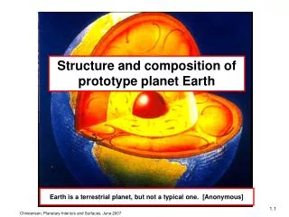
Structure and composition of prototype planet Earth. Earth is a terrestrial planet, but not a typical one. [Anonymous]. Internal structure from seismology. Fundamentals

Structure and composition of prototype planet Earth
E N D
Presentation Transcript
Structure and composition of prototype planet Earth Earth is a terrestrial planet, but not a typical one. [Anonymous]
Internal structure from seismology • Fundamentals • Seismic waves are generated by earthquakes, explosions, meteorite impacts, etc. With modern instruments, seismic waves generated by an earthquake of medium strength or an underground nuclear explosion can be recorded all over the globe. • P-waves (primary, longitudinal, acoustic wave): vp = [ (k+4/3μ) / ρ ]1/2 • S-waves (secondary, transversal): vs = [ μ / ρ ]1/2 • Rayleigh waves (like waves on water) • Love waves (shearing motion of surface) • Free oscillations are vibrations of the entire Earth (like ringing of a bell). They are excited (so that they are observable for up to a few days) by strong earthquakes. • Spheroidal modes 0S2 Toroidal modes 0T2 • Longest period (0S2) is 54 min. Periods depend on mode of oscillation and on elastic constants and density distribution in the whole Earth. }Body waves }Surface waves, dispersive [v depends on λ] Symbols: ρ – density, k – incompressibility, μ – shear modulus, λ – wavelength, v – seismic velocity, T -period
Registration of the San Francisco, 1906, Earthquake taken in Göttingen
Source Receiver Δ Seismic wave propagation through the Earth 2. Body wave propagation in a radially symmetric Earth Because v varies continuously with radius, body waves travel on curved paths. At seismic discontinuities: refraction, reflection, type conversion (S→P or P→S). Examples of nomenclature of waves: PP – once reflected at Earth‘s surface, PcP – reflected at core mantle boundary PKP – travelled as P-wave in core (Kern). • When v depends only on radius r, travel time T depends only on epicentral distance Δ. Found to be the case to first order (onion shell Earth). • Shadow zone for direct P-waves between Δ=103o and 142o: Evidence for core with reduced vp. • No S-waves observed in outer core liquid. • Weak arrivals (PKIKP) in shadow zone inner core (solid from free oscill. frequencies). • Knowledge of T(Δ) allows to determine epicenter location from three observations. • Inversion of T(Δ) allows to determine radial velocity structure vp(r) and vs(r) of the Earth. • Travel time data alone cannot constrain density ρ(r) [three unknowns in vp, vs: k, μ, ρ] Symbols: T - travel time, Δ – epicentral distance, r –radius from center of Earth, ρ - density
Reduced travel time T – 13 [sec/degr] Δ Shadow zone Δ in degrees Example of seismic recordings at different epicentral distances Recordings of an earthquake in Sumatra with standardized seismic instruments all over the world. The vertical component of ground motion is shown.
Free oscillations 1h 2h 3h 4h Recording of free oscillations, riding on top of the tidal wave, following the Chile 1960 earthquake. Theoretical variation of compressional energy density (full line) and shear energy density (broken line) with radius in the Earth for different oscillation modes. Note that the mode 10S2 has strong shear energy in the inner core (provided it is solid). Spectral analysis of several records like the one above. Each peak relates to an identifiable oscillation mode. Each observed eigenfrequency of an identified free oscillation mode puts constraints on Earth models [ k(r), μ(r), ρ(r) ] or [ v P(r), vs(r), ρ(r) ]. The modes carry information on ρ(r) in a way independent of how ρ enters into vp, vs. They therefore allow to constrain ρ(r). .
PREM: Preliminary Reference Earth Model Model based on the inversion of traveltimes of body waves and free oscillation frequencies. Subdivisions: Crust (variable, 6 - 40 km thick). Upper mantle (to 400 km depth). Transition Zone (400 – 700 km) with seismic discontinuities; main discontinuities at 410 km and 660 km depth. Lower Mantle 700 – 2890 km depth. Outer core 1220 – 3480 km radius. Inner core 0 – 1220 km radius.
Earth model: pressure, gravity, elastic constants k For known ρ(r), the variation of gravity g is μ Assuming that the pressure p is hydrostatic in the Earth, it is obtained from integrating dp/dr = -ρ(r)g(r) starting with p=0 at the Earth‘s surface. Gravity is nearly constant (≈ 10 m/s2) in the mantle. The incompressibly k increases with p, with little variation at core-mantle bound. Symbols: g – gravity acceleration, G – constant of gravity, p - pressure
Xenolith Composition of different parts of the Earth Sources of information: Crust – plenty of direct samples Upper Mantle – samples from exposed mantle rock or xenoliths (solid mantle rock carried upwards in volcanic vents) Deep mantle and core – indirect Mantle rock is rich in magnesium (over 90% consists of the elements Si, Mg, Fe, O). Crustal rocks are much less rich in Mg and comparatively more rich in Ca and Al. There is an increasing trend in the silicon content from mantle to oceanic crust to continental crust.
laser beam diamond saphir disk pressure chamber ruby powder Gasket sample diamond High pressure studies of Earth materials • In order to constrain the composition of the deep Earth, the properties (for example k, ρ) of candidate materials at high pressure (and temperature) must be studied. For this, three types of devices are in use: • Large volume press. Reaches pressures as at ~700 km depth in the Earth. Sample volume is a few mm3 at highest pressures. Electric heating allows to reach controlled high temperatures. • Diamond anvil press. Reaches pressures as in Earth‘s outer core. Sample size some ten μm. High temperatures by focussing a laser beam on a spot a few μm large. Allows in-situ observation and X-ray diffraction study of sample. • Shock wave experiments. Reaches pressures as in centre of Earth for μseconds. High temperature reached in shock wave. Observation of particle velocity and shock velocity allows to reconstruct properties such as pressure and density reached in shock. Diamond anvil press allows to gene-rate pressures as in the Earth‘s core
geotherm --- 660 km Ringwoodite 410 km Phase diagram of olivine (Mg0.9Fe0.1)2SiO4 At high pressure, olivine undergoes solid-solid phase changes (change in crystal structure) into more dense packages of the atoms: olivine (α) ↔ wadsleyite (β) ↔ ringwoodite (γ) ---------------- (Mg1-xFex)2SiO4 --------------- ↔ perovskite (pv) + magnesiowüstite (Mg1-yFey)SiO3 + (Mg1-zFez)O The α–β and the γ-pv+mw transitions are associated with a change in ρ, vp, vs on the order of 5-10%, the changes are smaller for the β-γ-transition. The transition pressure of the two main phase changes corresponds to a depth of ≈ 410 km and 660 km, respectively. The seismic discontinuities at these depths represent isochemical phase changes. The composition in the lower mantle is probably the same as in the upper mantle. The phase changes are mainly controlled by pressure, but depend also on temperature T. The Clapeyron slope dp/dT is positive for the α–β transition and negative for the γ-pv+mw transition. The seismically observed transition depths requires a temperature of order 1700-1800 K at 400-700 km depth.
Composition of Earth‘s core Results of shock wave measurements, plotted as bulk sound velocity Φ = (k/ρ)1/2 = (vp2- 4/3 vs2)1/2 versus density ρ. There is a systematic dependence on the atomic number. The seismically observed properties of the core agree nearly with those of iron, but the core density is slightly lower than that of pure iron (or an iron-nickel alloy). Elements such as chromium or manganese might fit better, but they are far too rare in the universe to make up the bulk of the core The core consists predominantly of iron (plus some nickel, whose properties are similar) and about 10% of a light element. Main candidates for the light element are S, Si and O. Sulphur dissolves well in liquid iron (as FeS), whereas FeO is not very soluable at low pressure (but might be at high p). The solid inner core is thought to be closer to pure Fe-Ni in composition than the outer core.
liquid melting temperature solid Temperatures in Earth‘s core Melting tempera-ture of iron as a function of pressure from experiments in a diamond anvil cell. An extrapolation to the pressure at the inner core boundary (3.3 Mbar) gives a temperature of about 5000 K. At the inner core boundary actual temperature and melting temperature coincide. The liquid outer core is assumed to be well mixed by convection. Here the temperature should follow an adiabatic gradient [dT/dp]adiab = αT/(ρcp). The melting point gradient is steeper than the adiabatic gradient. For this reason the core is solid at the centre and liquid further out (and not vice versa). As the Earth cools and the core temperature drops, the inner core grows by freezing iron to its surface. The light element(s) is (are) expelled in this process. Their concentration in the fluid layer surrounding the inner core therefore rises, making this layer buoyant. This drives compositional convection in the outer core. Symbols: α – thermal expansion coefficient, T – absolute temperature, cp – heat capacity at const. pressure
Plate tectonics and internal dynamics Earth is the only planet that shows (currently) plate tectonics, i.e. a permanent overturn of its oceanic parts and the drift of the continents. The rather stiff and brittle outer-most part of the mantle including the overlying crust is called the lithosphere. The lithosphere is broken up into a number of plates that move as nearly rigid units with respect to each other. Their typical thickness is about 100 km. The mantle below (asthenosphere) is solid, but soft enough to behave like a very viscous fluid on long time-scales. Oceanic lithosphere is continously created at mid-oceanic ridges. It is subducted and descends into the soft mantle at locations marked by deep sea trenches.
1000 1500 T[oC] liquid Solidus Liquidus 50 100 partially molten Lithospheric plate Basaltic crust Mantle plume Depth [km] Partial melting Rock rising below mid-oceanic ridge Crust formation and magnetic lineations at mid-oceanic ridges solid Plates diverge at mid-oceanic ridges. The „gap“ is filled by upwelling warm mantle rock, which eventually cools and is added to the plates. During adiabatic upwelling, the temperature crosses the solidus and partial melting (≈ 10%) occurs. The melt has a different composition (basaltic) than the source rock (peridotite). The melt is less dense, segregates upwards and cools at the surface to form basaltic oceanic crust ≈ 6 km thick. Basalt contains 1-3% ferromagnetic minerals (e.g. magnetite, Fe3O4). It is magnetized in the direction of the geomagnetic field when it cools below the Curie temperature. Earth‘s field reverses a few times in 1 Myr. Crust that has been magnetized when the field polarity was opposite (and has now moved away from the ridge) forms stripes with reduced total magnetic field. The observation of the magnetic stripes in the 1960s was the key for accepting plate tectonics and continental drift.
Plate motion from GPS measurements Plate boundaries are shown by black lines. The relative motion (change of distance) in mm/yr between GPS stations is shown, derived from measurements taken over a few years. The value in parantheses is the change from plate motion models based on geophysical data (i.e. dated magnetic lineations) covering several million years of time. The short-term motion agrees very well with that averaged over geological time.
Hotspots and mantle plumes Basaltic magmas also erupt in the interior of plates. Volcanic island chain with age progression away from the active volcanoes (Hawaii) Plate overrides fixed hotspot in the mantle. Mantle plumes: columns of upwelling rock (≈100 km diameter), 200-300oC warmer than ambient mantle. Originate at thermal boundary layer, perhaps above the core. Because of their excess temperature, plumes start to melt partially below the bottom of the plates (but not much deeper, slide 1.15). The solid part of the plume cannot penetrate into the stiff lithosphere and flattens below the plate. A third type of volcanic activity occurs near subduction zones. It is caused by H2O carried into the upper mantle by the descending plate. This reduces the solidus. The composition of these andesitic magmas is intermediate between that of basalt and continental crust.
Seismic tomography Most dynamical structures in the mantle below 100 km (plumes, subducted lithospheric slabs) have been originally inferred from indirect evidence. In the last 15 years, they have been mapped pro-gessively by seismic tomography. Seismic tomography uses small deviations from the expected travel times T(Δ), which are caused by deviations from a purely radial velocity structure vp(r), vs(r). Using many crossing ray paths, it is possible to identify and map the regions in the Earth where the seismic velocity is faster of slower than expected (for a given depth). Seismic velocity is sensitive to temperature (decreases with increasing temperature). Therefore seismically slow regions are usually associated with abnormally warm rock (plumes) and fast regions with cold material (e.g. subducted slabs). Seismic tomography is impeded by the uneven distribution of sources and receivers. The tomographic images are therefore somewhat blurred or may contain artefacts of the inversion.
Anomaly of P-wave velocity Seismic tomography: Example 1 Cross-section through a tomographic image of the mantle: Middle America and Carribean. The subducted Cocos plate approaches Middle America from the Pacific side and descends into the mantle, sinking to at least 1800 km depth.
Seismic tomography: Example 2 Seismic image of a plume in the upper mantle below the Eifel region (Western Germany). The plume rises from at least 400 km depth. Below that the resolution is lost because of the limited aperture of the array of seismic stations used in the experiment.