Download
1 / 19
190 likes | 342 Vues
Recent PM 2.5 Trends in Georgia. Andr é J. Butler Mercer University EVE 290L 14 April, 2008. Background. What is PM 2.5 ? Solid (or liquid) particles with aerodynamic diameters < 2.5 m m Why is the 2.5 m m distinction used?

E N D
Recent PM2.5 Trends in Georgia André J. Butler Mercer University EVE 290L 14 April, 2008
Background • What is PM2.5? • Solid (or liquid) particles with aerodynamic diameters < 2.5 mm • Why is the 2.5 mm distinction used? • Fine particles: insufficient inertia to deposit in nasal passages (imbed deep within lungs) • Toxicity: particles of this size contain chemicals that may be toxic
Background • What are the sources of PM2.5? • Anthropogenic • Primary: IC engines, fireplaces, meat-cooking operations, industrial processes • Secondary: atmospheric conversions of SO2 and NOx to SO42- and NO3-, respectively • Biogenic • Primary: volcanoes, soil erosion, sea spray • Secondary: atmospheric conversion of organic gases to particulate organic carbon
Background • What are the effects of PM2.5? • Environmental impacts • Climate change (cooling) • Visibility degradation • Human health impacts • Morbidity (decreased lung function, increased respiratory hospitalizations, school absenteeism) • Mortality (cancer, cardiac arrest)
Temporal Analysis of PM2.5 Mass Data • Summary statistics
Temporal Analysis of PM2.5 Mass Data • Weekly-averaged and seasonal trends in PM2.5 mass (a) Weekly-averaged trends in PM2.5 mass (b) Seasonal variations in PM2.5 mass
PM2.5 Mass Results • Temporal • Highest values in summer • Lowest values on Monday • Highest values at night and AM rush • Spatial • Overall, little spatial variation
Temporal Analysis of SO42- • Seasonal SO42- variations and Spearman rank correlation coefficient matrix Sulfate R-values Sulfate R-values Summary statistics
Temporal Analysis of NH4+ • Seasonal NH4+ variations and Spearman rank correlation coefficient matrix Ammonium R-values Summary statistics
Temporal Analysis of NO3- • Seasonal NO3- variations and Spearman rank correlation coefficient matrix Nitrate R-values Summary statistics
Major Ionic Species Results • SO42- • Peak values in summer • Highest when wind from west (180-360) • Spatially homogeneous • NO3- • Peak values in winter • Spatially homogeneous • NH4+ • Peak values in summer • Associated with SO42- and NO3- • Spatially homogeneous
Temporal Analysis of OC • Seasonal OC variations and Spearman rank correlation coefficient matrix OC R-values Summary statistics
Temporal Analysis of EC • Seasonal EC variations and Spearman rank correlation coefficient matrix EC R-values Summary statistics
Indicators of Secondary Aerosol Production • Total carbon (TC=OC+EC) to EC ratio
Estimation of Secondary Aerosol Production • Method of Turpin and Huntzicker (1991) and Castro et al. (1999) OCsec = OCtot – OCpri OCpri = EC(OC/EC)pri OCsec = secondary OC OCtot = total OC OCpri = primary OC (OC/EC)pri = primary ratio estimate
OC/EC Results • Organic carbon • Peak values in summer • Lowest values on Monday • Significant secondary contribution (43-80%) • Spatially homogeneous • Elemental carbon • Peak values in summer (August anomaly) • Lowest values on weekends
Predicting PM2.5 Spatially-averaged model for Case 3: R2 = 0.63
Conclusions • Temporal variation in PM2.5 concentrations greater than spatial • Mean 24-hour levels: 19.3 - 21.2 mg/m3 • Annual NAAQS: 15 mg/m3 (3 yrs data) • Peak levels in summer (mass and all species except NO3-) • August 1999 was anomalous • Slight increase in PM2.5 during work week • Late-night, early-morning diurnal peaks
Conclusions, continued • Major ions accounted for ~40% of mass • OC largest single species (~31% of mass) • Secondary formation important (43-79%)