Download
1 / 19
200 likes | 308 Vues
Learn the fundamentals of Reinforcement Learning (RL) including Agent-Environment Interaction, Markov Decision Processes, Value Functions, and Bellman Equations. Understand the RL problem, idealized form, and mathematical components. Explore policy definitions, learning methods, algorithm design, state-action dynamics, and rewards. Discover the goals, returns, discounting rates, and episodic tasks in RL. Dive into examples and distinctions in RL tasks for comprehensive understanding.

E N D
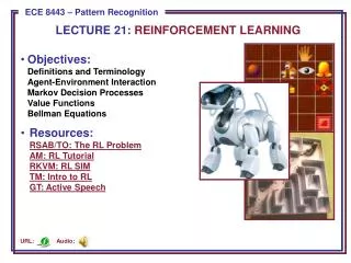
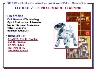
LECTURE 25: REINFORCEMENT LEARNING • Objectives:Definitions and TerminologyAgent-Environment InteractionMarkov Decision ProcessesValue FunctionsBellman Equations • Resources:RSAB/TO: The RL ProblemAM: RL TutorialRKVM: RL SIMTM: Intro to RLGT: Active Speech
Attributions • These slides were originally developed by R.S. Sutton and A.G. Barto, Reinforcement Learning: An Introduction. (They have been reformatted and slightly annotated to better integrate them into this course.) • The original slides have been incorporated into many machine learning courses, including Tim Oates’ Introduction of Machine Learning, which contains links to several good lectures on various topics in machine learning (and is where I first found these slides). • A slightly more advanced version of the same material is available as part of Andrew Moore’s excellent set of statistical data mining tutorials. • The objectives of this lecture are: • describe the RL problem; • present idealized form of the RL problem for which we have precise theoretical results; • introduce key components of the mathematics: value functions and Bellman equations; • describe trade-offs between applicability and mathematical tractability.
r r r . . . . . . t +1 t +2 s s t +3 s s t +1 t +2 t +3 a a a a t t +1 t +2 t t +3 The Agent-Environment Interface
The Agent Learns A Policy • Definition of a policy: • Policy at state t, πt, is a mapping from states to action probabilities. • πt (s,a)= probability that at = a when st = s. • Reinforcement learning methods specify how the agent changes its policy as a result of experience. • Roughly, the agent’s goal is to get as much reward as it can over the long run. • Learning can occur in several ways: • Adaptation of classifier parameters based on prior and current data (e.g., many help systems now ask you “was this answer helpful to you”). • Selection of the most appropriate next training pattern during classifier training (e.g., active learning). • Common algorithm design issues include rate of convergence, bias vs. variance, adaptation speed, and batch vs. incremental adaptation.
Time steps need not refer to fixed intervals of real time (e.g., each new training pattern can be considered a time step). Actions can be low level (e.g., voltages to motors), or high level (e.g., accept a job offer), “mental” (e.g., shift in focus of attention), etc. Actions can be rule-based (e.g., user expresses a preference) or mathematics-based (e.g., assignment of a class or update of a probability). States can be low-level “sensations”, or they can be abstract, symbolic, based on memory, or subjective (e.g., the state of being “surprised” or “lost”). States can be hidden or observable. A reinforcement learning (RL) agent is not like a whole animal or robot, which consist of many RL agents as well as other components. The environment is not necessarily unknown to the agent, only incompletely controllable. Reward computation is in the agent’s environment because the agent cannot change it arbitrarily. Getting the Degree of Abstraction Right
Is a scalar reward signal an adequate notion of a goal? Perhaps not, but it is surprisingly flexible. A goal should specify what we want to achieve, not how we want to achieve it. A goal must be outside the agent’s direct control — thus outside the agent. The agent must be able to measure success: explicitly frequently during its lifespan. Goals
Returns • Suppose the sequence of rewards after step t is rt+1, rt+2,… What do we want to maximize? • In general, we want to maximize the expected return, E[Rt], for each step t, where Rt = rt+1 + rt+2 + … + rT, where T is a final time step at which a terminal state is reached, ending an episode. (You can view this as a variant of the forward backward calculation in HMMs.) • Here episodic tasks denote a complete transaction (e.g., a play of a game, a trip through a maze, a phone call to a support line). • Some tasks do not have a natural episode and can be considered continuing tasks. For these tasks, we can define the return as: • where γis the discounting rate and 0 ≤ γ ≤ 1. γclose to zero favors short-term returns (shortsighted) while γclose to 1 favors long-term returns. γcan also be thought of as a “forgetting factor” in that, since it is less than one, it weights near-term future actions more heavily than longer-term future actions.
Example • Goal: get to the top of the hill as quicklyas possible. • Return: • Reward = -1 for each step taken when you are not at the top of the hill. • Return = -(number of steps) • Return is maximized by minimizing the number of step to reach the top of the hill. • Other distinctions include deterministic versus dynamic: the context for a task can change as a function of time (e.g., an airline reservation system). • In such cases time to solution might also be important (minimizing the number of steps as well as the overall return).
In episodic tasks, we number the time steps of each episode starting from zero. We usually do not have to distinguish between episodes, so we write st,j instead of st for the state s at step t of episode j. Think of each episode as ending in an absorbing state that always produces reward of zero: We can cover all cases by writing: where γ= 1 only if a zero reward absorbing state is always reached. A Unified Notation r1 = +1 r2 = +1 r3 = +1 r4 = 0 r5 =0 … s0 s1 s2
“The state” at step t refers to whatever information is available to the agent at step tabout its environment. The state can include immediate “sensations,” highly processed sensations, and structures built up over time from sequences of sensations. Ideally, a state should summarize past sensations so as to retain all “essential” information, i.e., it should have the Markov Property: for all s’, r, and histories st, at, rt, st-1, at-1, …, r1, s0, a0. If a reinforcement learning task has the Markovian property, it is basically a Markov Decision Process (MDP). If state and action sets are finite, it is a finite MDP which consists of the usual parameters for a Markov model: The transition probability is given by: and a slightly modified expression for the output probability at a state, called the reward probability in this context: Markov Decision Processes
At each step, robot has to decide whether it should: actively search for a can, wait for someone to bring it a can, or go to home base and recharge. Searching is better but runs down the battery; if runs out of power while searching, it has to be rescued (which is bad). Decisions made on basis of current energy level: high, low. Reward = number of cans collected. Example: Recycling Robot
The value of a state is the expected return starting from that state; depends on the agent’s policy: The value of taking an action in a state under policy p is the expected return starting from that state, taking that action, and thereafter followingp: Value Functions
Bellman Equation for a Policy • The basic idea: • So: • Or, without the expectation operator: • This is a set of linear equations, one for each state. This reduces the problem of finding the optimal state sequence and action to a graph search:
For finite MDPs, policies can be partially ordered: There is always at least one (and possibly many) policy that is better than or equal to all the others. This is an optimal policy. We denote them all p *. Optimal policies share the same optimal state-value function: Optimal policies also share the same optimal action-value function: This is the expected return for taking action a in state s and thereafter following an optimal policy. Optimal Value Functions
Bellman Optimality Equation for V* • The value of a state under an optimal policy must equalthe expected return for the best action from that state: • V* is the unique solution of this system of nonlinear equations. • The optimal action is again found through the maximization process: • Q* is the unique solution of this system of nonlinear equations.
Finding an optimal policy by solving the Bellman Optimality Equation requires the following: accurate knowledge of environment dynamics; we have enough space an time to do the computation; the Markov Property. How much space and time do we need? polynomial in number of states (via dynamic programming methods); BUT, number of states is often huge (e.g., backgammon has about 10**20 states). We usually have to settle for approximations. Many RL methods can be understood as approximately solving the Bellman Optimality Equation. Solving the Bellman Optimality Equation
Q-learning is a reinforcement learning technique that works by learning an action-value function that gives the expected utility of taking a given action in a given state and following a fixed policy thereafter. A strength with Q-learning is that it is able to compare the expected utility of the available actions without requiring a model of the environment. The value Q(s,a) is defined to be the expected discounted sum of future payoffs obtained by taking action a from state s and following an optimal policy thereafter. Once these values have been learned, the optimal action from any state is the one with the highest Q-value. The core of the algorithm is a simple value iteration update. For each state, s, from the state set S, and for each action, a, from the action set A, we can calculate an update to its expected discounted reward with the following expression: where rt is an observed real reward at timet, αt(s,a) are the learning rates such that 0 ≤ αt(s,a) ≤ 1, and γ is the discount factor such that 0 ≤ γ < 1. This can be thought of as incrementally maximizing the next step (one look ahead). May not produce the globally optimal solution. Q-Learning* * From Wikipedia (http://en.wikipedia.org/wiki/Q-learning)
Summary • Agent-environment interaction (states, actions, rewards) • Policy: stochastic rule for selecting actions • Return: the function of future rewards agent tries to maximize • Episodic and continuing tasks • Markov Property • Markov Decision Process • Transition probabilities • Value functions • State-value function for a policy • Action-value function for a policy • Optimal state-value function • Optimal action-value function • Optimal value functions • Optimal policies • Bellman Equations • The need for approximation • Other forms of learning such as Q-learning.