Download

1 / 28
360 likes | 704 Vues
Bézier Curves. Representing free-form shape. CAD/CAM software requires shape to be represented mathematically Standard mathematical representations such as y=f(x) very problematic Overcome using parametric representations. The simplest parametric curve. The Line: L (p) = (1-p) L 0 + p L 1

E N D
Representing free-form shape • CAD/CAM software requires shape to be represented mathematically • Standard mathematical representations such as y=f(x) very problematic • Overcome using parametric representations
The simplest parametric curve • The Line: • L(p) = (1-p)L0 + pL1 • 0 p 1 L1 L(p) L0
The simplest parametric curve • The Line: • L(p) = (1-p)L0 + pL1 • 0 p 1 L1 L0 L(0.0)
The simplest parametric curve • The Line: • L(p) = (1-p)L0 + pL1 • 0 p 1 L1 L(0.2) L0
The simplest parametric curve • The Line: • L(p) = (1-p)L0 + pL1 • 0 p 1 L1 L(0.4) L0
The simplest parametric curve • The Line: • L(p) = (1-p)L0 + pL1 • 0 p 1 L1 L(0.6) L0
The simplest parametric curve • The Line: • L(p) = (1-p)L0 + pL1 • 0 p 1 L1 L(0.8) L0
The simplest parametric curve • The Line: • L(p) = (1-p)L0 + pL1 • 0 p 1 L1 L(1.0) L0
The simplest parametric curve • The Line: • L(p) = (1-p)L0 + pL1 • 0 p 1 • Note that every point we evaluate on the curve is constructed as a weighted average of the two end points
1 • L(p) = bi,1(p) Li i=0 The simplest parametric curve • We can reformulate the equation for a line: • b0,1(p) = (1-p) • b1,1(p) = p 0 p 1
1 • L(p) = bi,1(p) Li i=0 The simplest parametric curve • We can reformulate the equation for a line: • b0,1(p) = (1-p) • b1,1(p) = p 0 p 1 Weighing for each point: Basis Function (in p)
1 • L(p) = bi,1(p) Li i=0 The simplest parametric curve • We can reformulate the equation for a line: • b0,1(p) = (1-p) • b1,1(p) = p 0 p 1 Weighing for each point: Basis Function (in p) Index
1 • L(p) = bi,1(p) Li i=0 The simplest parametric curve • We can reformulate the equation for a line: • b0,1(p) = (1-p) • b1,1(p) = p 0 p 1 Weighing for each point: Basis Function (in p) Index Degree
n • C(u) = bi,n(u) Ci i=0 General parametric curve • Generalise the formulation: • Ci = [xi, yi, zi] • Shape depends on: • Degree, n • Position of Control Points,Ci • Choice of Basis functions,bi,n(u) 0 u 1
Cubic Bezier curve C3 C1 C(u) C2 C0
Cubic Bezier curve C3 C1 Cubic: n=3 (n+1) Control Points C(u) C2 C0
Cubic Bézier curve C3 C1 Control Polygon C(u) C2 C0
Illustration of changing: • Degree, n • Position of Control Points,Ci • Choice of Basis functions,bi,n(u)
n • C(u) = bi,n(u) Ci i=0 Bézier curve 0 u 1 • Each point on the curve is made up of a weighted average of the control points. • Weightings given by the Basis functions,bi,n(u)
n • C(u) = bi,n(u) Ci i=0 Bézier basis functions 0 u 1 • bi,n(u) = nCi (1-u)n-i ui • nCi = n! (n-i)! i!
nCi = n! (n-i)! i! Cubic Bézier basis functions bi,n(u) = nCi (1-u)n-i ui
bi,3(u) 1.0 b0,3(u) b3,3(u) 0.666 b1,3(u) b2,3(u) 0.333 0.0 u 0.0 0.333 0.666 1.0 Cubic Bézier basis functions
bi,3(u) 1.0 b0,3(u) b3,3(u) 0.666 b1,3(u) b2,3(u) 0.333 0.0 u 0.0 0.333 0.666 1.0 Cubic Bézier basis functions • Sum of all basis functions is always equal to 1.0 for any u
bi,3(u) 1.0 b0,3(u) b3,3(u) 0.666 b1,3(u) b2,3(u) 0.333 0.0 u 0.0 0.333 0.666 1.0 Cubic Bézier basis functions • C(0)C0 • C(1)Cn
Advantages of Bézier Curves: • Start and End on the first and last control points • Tangents defined by second and penultimate control points – can piece several curves together with tangent continuity
Advantages of Bézier Curves: • The shape of the curve roughly corresponds to the shape of the control polygon – not true of other basis functions • They are mathematically stable and well defined • They are invariant under control point transformations – to transform the curve just transform the control polygon
Advantages of Bézier Curves: • The maximum and minimum values in any direction are given by the bounding box. This is the smallest box that contains the control polygon.