Density Curves
Density Curves. Henry Mesa. Use your keyboard’s arrow keys to move the slides forward ( ▬►) or backward ( ◄▬) Use the (Esc) key to exit. What is a density curve? . A good question. Density curves represent “idealized” distributions. What do you mean idealized?.

Density Curves
E N D
Presentation Transcript
Density Curves Henry Mesa Use your keyboard’s arrow keys to move the slides forward (▬►) or backward (◄▬) Use the (Esc) key to exit
What is a density curve? A good question. Density curves represent “idealized” distributions. What do you mean idealized? Now we are going into the realm of philosophy. Since we are applying mathematics, when you apply something, the field of philosophy comes into play that guides us as to how one can apply something. What are the characteristics of the “population that we are studying” that would produce the type of numbers that we are measuring? Suppose 30 students are given a coin, and asked to flip it 20 times, and record the number of times a tails appears out of the 20 throws. Here are the results from this situation. For example one student got four tails, and one student got 14 tails.
Suppose we asked another 30 students to do the same thing. Here is the result from those 30 students. And we do it again. And here is the result from this attempt. Each time we get a different result. What we need is to understand the basic mechanism that creates these numbers. Density curves are the result of mathematicians creating different characteristics and then seeing what type of numbers are produced by these characteristics.
Here is a very simple example of an idealized number. If I flip a fair coin, what is the probability that it lands heads? Go ahead, I will give you a second. Do you think you have it? Yes you are correct 20%. Shook you up a bit I bet. Yes, it is 50%, but why do you say that? Where did you get that 50% from? Have you ever tested it? And what do you mean by 50% (a question for a later date)? • I am assuming that you came up with the 50% because you thought to yourself: • The coin has only two sides. • I will ignore or assume that the chance of the coin landing on its side is so small as to be virtually impossible. • Neither side is more equally likely to show up than the other; coin is perfectly balanced. • There is no trickery going on when the coin is being flipped; a totally random throw. This is what I mean by idealized. I came up with the above criteria without ever flipping the coin.
Furthermore, I can use that idealized number to create a model that will mimic what might occur when I do flip the coin in reality. I am sure you have seen this type of device where balls are dropped from a position and then the ball hits a series of pegs until they reach a tube. The balls then accumulate in the tube. The picture below I got from, http://www.ms.uky.edu/~mai/java/stat/GaltonMachine.html We will soon see that this type of scenario is modeled by the idealized distribution below. You will create this theoretical curve later.
To reiterate, the histograms shown earlier, are the result of thirty students flipping a coin 20 times and then recording (the measurement) how many tails they got. Then repeating the process with another thirty students and so on. Those numbers where generated from the idealized distribution shown here; at least in theory. Please think about what I have just presented. If you get it, and accept it, then you are on your way to understanding this material.
Now, we are ready to continue. We have some idea of how an idealized curve can be created. Density curves come from measurements that are quantitative, and furthermore, continuous. Is this important? Yes. I have often tried to ignore this issue at this point only to have my more creative students, well, get too creative. Basically, they ignore what I have told them to do , and think that they can do the same thing by making an incorrect assumption. At issue is continuity. You will point out to me later if I have made a mistake by introducing this now or not. At least by introducing it you will have some idea that this is an important issue. Quantitative data comes in two basic types: discrete and continuous. Think back to my coin example. In this scenario I had students count how many tails they got. This is an example of a discrete measurement. Why?
Danger! We are now going into deep mathematical philosophy mode. Hang on. When I was first introduced to numbers as a child, as were you, I was introduced to discrete numbers: 1, 2, 3, 4, 5, 6, 7, … As far as I new, there was no such thing as 1.5, nor 3.5 for example. Does that mean that fractions are not discrete? No, hang on. Here I have happy faces. These are three distinct happy faces. Even if I put them as close as possible, we have three happy faces.
If my measurements are discrete, I should be able to create an interval around each measurement such that no other measurement is found in that interval. An example of a discrete measurement occurs if my measurements are integers: {…-3, -2, -1, 0, 1, 2, 3, …}. I can then create an interval around each number so that there is no other measurement value inside that interval. ( ) ( ) ( ) ( ) This is not possible if my measurements are continuous. Suppose that my measurements can take on any real number between -4 and 4. Since I have a continuous measurement then any time I create an interval around any number, there is another possible measurement inside that interval. -4.0000000000000345 inside interval. ( )
Now measuring devices are thought of as discrete, but it does not mean that what they are measuring is discrete. I will use the most incomprehensible concept that mankind has had to deal with as the example of a continuous system. TIME Is time continuous or discrete? I think of it as continuous; after all I view the world as moving, changing in a continuous manner. When I get up and cross the room, I must pass through every portion of the room to get from point A to point B. I view time as being continuous as well for that reason, I think. But our measuring machines are all discrete in nature. The sun dial is the only measuring machine of time that moves continuously as does time (I am assuming that this is the case with time. I could be wrong).
Think about how the shadow crosses the disk. To go from one spot to an ending spot I must traverse every single space of the disk, which the spaces represents the measurement. And for any single measurement, no matter how small I make the interval around it, I still have some other measurement value inside it.
Here is a simple discrete example. Consider the measurement resulting from tossing a fair six-sided die. What are the possible measurements? I hope you said the values {1, 2, 3, 4, 5, 6}. Now what are the frequencies of those numbers? 1/6 Below is the graph of this situation.
Similarly, here is an example of a continuous scenario. Excel can create random numbers using a pseudo-random number generator. These random number generators are used in a variety of scientific, and not so scientific endeavors. For example random number generators are used to create realistic computer generated scenes in the movies today. The continuous version of the die problem is the uniform distribution. The graph is shown below. If I set the random number generator to provide me with real numbers between 1 and 6 from a uniform distribution then, I can get a value such as 1.67980045032119, while a die can only give me numbers such as 1, 3, 6, and so on.
The uniform density curve is one example of a density curve, and it is the simplest. Here are some facts about any density curve. 1. The data they represent is continuous. 2. The area underneath the curve is always one square unit. 1 1 Area = = 1 Area = (6 – 1) = 1 (b – a) (b – a) (6 – 1) The next examples will only use the uniform distribution.
What is the height of the uniform distribution shown below? Area = 1= (18 – 10) (?) 1 Height = 8
What is the height of the uniform distribution shown below? Area = 1= (26 – 3) (?) 1 Height = 23
Function Notation We are going to be communicating the calculation of relative frequencies, which later we will call probabilities using function notation. I will expect that as you write down steps you will write them down correctly using appropriate syntax. What you write down must make sense otherwise points will be deducted from your answers. In algebra you encountered the notation f(x) = y that denotes my equation is a function. We will use the notation P(some measurement) = relative frequency, which states our function calculates the relative frequency of some defined measurement. Let us see how this works.
Excel’s random number generator is set to produce numbers from 3 to 26. How often will I get a number less than 8? What follows are the steps you are to carry out regardless of how you view this; meaning even if you see the answer, I am expecting you to do this exactly. 1. Create a picture of the distribution, label everything; notice I called the horizontal axis X. 2. Mark the region on the x-axis pertaining to the measurement in question. Do not worry about making this exactly proportional. 3. Shade in the area that depicts the relative frequency. Remember that the area underneath that curve represents, relative Frequency (how often something occurs). 4. Now use function notation to describe what you are trying to do. P(X < 8) = 8 5. Lastly, find your answer. Your written work should look exactly like this. No deviations from this process. P(X < 8) = (8 – 3) = 0.2174
Excel’s random number generator is set to produce numbers from 3 to 26. How often will I get a number greater than 20? On your own piece of paper carry out the steps as done in the previous exercise. Then click forward to see the answer, and the steps. 20 Your written work should look exactly like this. No deviations from this process. P(X > 20) = (26 – 20) = 0.2609
Excel’s random number generator is set to produce numbers from 3 to 26. How often will I get a number between 12 and 18? On your own piece of paper carry out the steps as done in the previous exercise. Then click forward to see the answer, and the steps. 12 18 Your written work should look exactly like this. No deviations from this process. P(12 < X < 18) = (18 – 12) = 0.2609
Excel’s random number generator is set to produce numbers from 3 to 26. How often will the number 12 appear? On your own piece of paper carry out the steps as done in the previous exercise. Then click forward to see the answer, and the steps. P(X = 12) = (12 – 12) = 0 A major consequence of continuous measurements is that the chance, relative frequency, we will give to a single value appearing is zero. Why? 12 To understand this, think about the die problem. What is the proportion of times, relative frequency, that a four appears? P(a four appears) = 1/6. We say this because a die has six sides all equally likely, and only one side has a four on it.
Now consider the same scenario but in a continuous setting. I set Excel’s random number generator to produce any real number between 1 and 6. How often will the random number generator produce a 4? If you think of this as a die situation, how many sides does this die have? Infinitely many sides, meaning the number of numbers between 1 and 6 are infinitely many. The proportion of times that we will get one number out of an infinite set of possible values will be defined as zero. P(a four appears) = (4 - 4)(1/5) = 0
Study this as often as you need. The ideas presented here will be the norm in MTH 243 and MTH 244. Knowing these ideas well will make the material in this course easier to understand. The next density curve we will study is the normal density curve. Out of all the possible density curves this is very special. Study Hard.