Density Curves and Normal Distributions

Density Curves and Normal Distributions

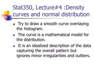
Density Curves • So far we have worked only with jagged histograms and stem plots to analyze data • As we begin to explore more fully the many statistical calculations and analyses one can perform on data it will become clear that working with smooth curves is much easier than jagged histograms

Density Curves Continued… • A density curve is a smooth curve that describes the overall pattern of a distribution by showing what proportions of observations (not counts) fall into a range of values.

Density Curves Continued… • Areas under a density curve represent proportions of observations • The scale of a density curve is adjusted in such a way that the total area under the curve is always equal to 1

Mean and Median of Density Curves • Median: The point which divides the area under the curve in half • Mean: The point at which the curve would balance if made out of solid material

For a symmetric Density curve… For a skewed density curve…

Constructing a simple density curve for dice simulation… • We will simulate rolling a 6 sided die 120 times using the command randInt(1,6,120) L2 2) 3)

Though our histogram looks jagged, we can approximate this histogram using a density curve: 20 1 2 3 4 5 6 1 2 3 4 5 6

6 Based on the density curve above what proportion of outcomes fall within the following intervals:

Normal Curves • A Particularly important class of density curves • Symmetric, single peak, bell shape • The mean of a density curve (including the normal curve) is denoted by and the standard deviation is denoted by • All Normal distributions have the same overall shape. Any differences can be explained by and

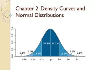
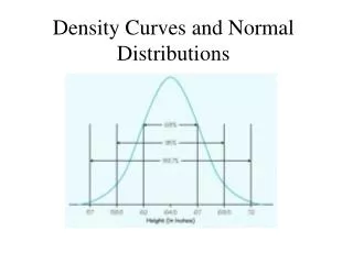
The 68–95–99.7 RULE In a normal distribution with mean and standard deviation : - 68% of the observations fall within of the mean - 95% of the observations fall within of the mean - 99.7% of the observations fall within of the mean

Percentiles The percentile of a score, x, is the percentage of scores which fall at or below the score. Pk = Score at the kth percentile rank.

Example: If you scored an 89 on a recent statistics test, and the other scores in the class are listed below: a) what is your percentile ranking? b) What is P40 Scores on test: 29, 45, 50, 69, 70, 70, 71, 80, 83, 84, 88, 89, 89, 90, 91, 93, 95, 98, 99, 100

Standard Normal Calculations Often times we are asked to compare the scores of two pieces of data that do not come from the same distribution. In order to decide which score is in fact higher, we must first standardize the scores If x is an observation from a distribution that has A mean and a standard deviation then the standardize value of x (often called the z-score) is:

The z-score tells us how many standard deviations a particular piece of data is away from the mean of the distribution. It therefore allows us to make comparisons across distributions: Example: Let’s say I gave two tests. On test 1 the mean was 68 and the standard deviation was 10. On test two the mean was 85, and the standard deviation was 4. A student who in the first test got a score of 83 claims that, relatively speaking, his score is better than a score of 87 received by his friend on test 2. Is he right? (assume both tests had approximately bell shaped distributions)

Density Curves and Normal Distributions