Optimization Techniques for Efficient DSP Programming on StarCore SC140
This document explores optimization techniques for DSP programming using the C language, specifically targeting the StarCore SC140 architecture. It covers key concepts such as compiler extensions, coding styles, and recommendations for improving code efficiency. By ensuring reductions in cycle counts, code sizes, and power consumption, developers can achieve optimal performance. The discussion also addresses C's abilities and limitations in handling digital signal processing tasks, emphasizing techniques like intrinsics and pragmas that facilitate efficient coding practices.

Optimization Techniques for Efficient DSP Programming on StarCore SC140
E N D
Presentation Transcript
C Optimization Techniques for StarCore SC140 Created by Bogdan Costinescu
Agenda • C and DSP Software Development • Compiler Extensions for DSP Programming • Coding Style and DSP Programming Techniques • DSP Coding Recommendations • Conclusions
What do optimizations mean? • reduction in cycle count • reduction in code size • reduction in data structures • reduction in stack memory size • reduction of power consumption • how do we measure if we did it right?
Why C in DSP Programming? • C is a "structured programming language designed to produce a compact and efficient translation of a program into machine language” • high-level, but close to assembly • large set of tools available • flexible, maintainable, portable => reusability
Compiler-friendly Architectures • large set of registers • orthogonal register file • flexible addressing modes • few restrictions • native support for several data types
Example - StarCore SC140 • Variable Length Execution Set architecture • one execution set can hold up to: • four DALU instructions • two AGU instructions • scalable architecture with rich instruction set • large orthogonal register file • 16 DALU • 16 + 4 + 4 AGU • short pipeline => few restrictions • direct support for integers and fractionals
Is C a Perfect Match for DSPs? • fixed-point not supported • no support for dual-memory architectures • no port I/O or special instructions • no support for SIMD instructions • vectors represented by pointers
C Support for Parallelism • basically, NONE • C = a sequential programming language • cannot express actions in parallel • no equivalent of SIMD instructions • the compiler has to analyze the scheduling of independent operations • the analysis depends on the coding style
Can C be made efficient for DSPs? YES, IF the programmer understands • compiler extensions • programming techniques • compiler behavior
Compiler Extensions • intrinsics • access efficiently the target instruction set • new data types • use processor-specific data formats in C • pragmas • providing extra-information to the compiler • inline assembly • the solution to “impossible in C” problem
Intrinsic functions (Intrinsics) • special compiler-translated function calls • map to one or more target instructions • extend the set of operators in C • define new types • simple and double precision fractional • extended precision fractionals • emulation possible on other platforms
Data Types • DSPs may handle several data formats • identical with C basic types • integers • common length, but different semantics • fractionals on 16 and 32 bits • particular DSP (i.e. including the extension) • fractionals on 40 bits • all DSP specific data types come with a set of operators
C Types for Fractionals • conventions: • Word16 for 16 bit fractionals • Word32 for 32 bit fractionals • Word40 for 40 bit fractionals (32 bits plus 8 guard bits) • Word64 for 64 bit fractionals (not direct representation on SC140) • intrinsics, not conventions, impose the fractional property on values
Fractional Emulation • needed on non-StarCore platforms • maintain the meaning of fractional operations • in some limit cases, the emulated results are not correct • e.g. mpysu uses 32-bits for results plus sign • special Metrowerks intrinsics to solve possible inconsistencies • e.g. mpysu_shr16
Fractional Values and Operators • introduced by fractional intrinsics • operators standardized (ITU-T, ETSI) • addition, multiplication • saturation, rounding • scaling, normalization • operate on specific data types Word16 add(Word16, Word16); Word32 L_add(Word32, Word32); Word40 X_add(Word40, Word40); Word64 D_add(Word64, Word64);
Pragmas • standard mode to speak with compilers • describe code or data characteristics • pragmas do not influence the correctness • but influence significantly the performance #pragma align signal 8 #pragma loop_unroll 4 #pragma inline #pragma loop_count (20, 40, 4)
Alignment pragma • #pragma align *ptr 8 • for parameters • #pragma align ptr 8 • for vector declaration and definition • derived pointers may not inherit the alignment Word16 *p = aligned_ptr + 24; /* not recommended */ #define p (aligned_ptr + 24) /* recommended */ • create a new function if you want to specify alignment for internal pointers
Inline Assembly • whole functions • only one instruction • asm(“ di”); • difficult access to local function symbols • global can be accessed by their name • the asm statements block the C optimization process
Inline Assembly • access to special target features not available through intrinsics • special calling convention • the programmer has more freedom • fast assembly integration with C • easy integration of legacy code • two types • one instruction, e.g. asm(“ di"); • a whole function
Inline Assembly - Example asm Flag GetOverflow(void) { asm_header return in $d0; .reg $d0,$d1; asm_body clr d0 ; extra cycle needed to allow DOVF to ; be written even by the instructions ; in the delay slot of JSRD bmtsts #$0004,EMR.L ; test the Overflow bit from EMR move.w #1,d1 tfrt d1,d0 ; if Overflow return 1, else return 0 asm_end }
Compiler Optimizations • standard C optimizations • low level (target) optimizations • several optimization levels available • fastest code • smallest code • global optimizations • all files are analyzed as a whole • the best performance
DSP Application Success Factors • high-performance, compiler-friendly target • good optimizing compiler • good C coding style in source code => the only factor tunable by the programmer is the C coding style • coding style includes programming techniques • no compiler can defeat from GIGO
Programming Techniques • described in the compiler’s manual • styles to be used • pitfalls to be avoided • explicitly eliminate data dependencies • complement compiler’s transformations that restructure the code
SC140 Programming Techniques • general DSP programming techniques • loop merging • loop unrolling • loop splitting • specific to StarCore and its generation • split computation • multisample
Loop Merging • combines two loops in a single one • precondition: the same number of iterations • may eliminate inter-loop storage space • increases cache locality • decreases loop overhead • increases DALU usage per loop iteration • typically, reduces code size
Loop Merging Example /* scaling loop */ for ( i = 0; i < SIG_LEN; i++) { y[i] = shr(y[i], 2); } /* energy computation */ e = 0; for ( i = 0; i < SIG_LEN; i++) { e = L_mac(e, y[i], y[i]); } /* Compute in the same time the */ /* energy of the scaled signal */ e = 0; for (i = 0; i < SIG_LEN; i ++) { Word16 temp; temp = shr(y[i], 2); e = L_mac(e, temp, temp); y[i] = temp; }
Loop Unrolling • repeats the body of a loop • increases the DALU usage per loop step • increases the code size • depends on • data dependencies between iterations • data alignment of implied vectors • register pressure per iteration • number of iterations to be performed • keeps the bit-exactness
Loop Unrolling Example int i; Word16 signal[SIGNAL_SIZE]; Word16 scaled_signal[SIGNAL_SIZE]; /* ... */ for(i=0; i<SIGNAL_SIZE; i++) { scaled_signal[i] = shr(signal[i], 2); } /* ... */ int i; Word16 signal[SIGNAL_SIZE]; #pragma align signal 8 Word16 scaled_signal[SIGNAL_SIZE]; #pragma align scaled_signal 8 /* ... */ for(i=0; i<SIGNAL_SIZE; i+=4) { scaled_signal[i+0] = shr(signal[i+0], 2); scaled_signal[i+1] = shr(signal[i+1], 2); scaled_signal[i+2] = shr(signal[i+2], 2); scaled_signal[i+3] = shr(signal[i+3], 2); } /* ... */
Compiler generated code ; With loop unrolling : 2 cycles inside ; the loop. ; The complier uses software pipelining [ move.4f (r0)+,d0:d1:d2:d3 move.l #_scaled_signal,r1 ] [ asrr #<2,d0 asrr #<2,d3 asrr #<2,d1 asrr #<2,d2 ] loopstart3 [ moves.4f d0:d1:d2:d3,(r1)+ move.4f (r0)+,d0:d1:d2:d3 ] [ asrr #<2,d0 asrr #<2,d1 asrr #<2,d2 asrr #<2,d3 ] loopend3 moves.4f d0:d1:d2:d3,(r1)+ ; Without loop unrolling : 6 cycles ; inside the loop loopstart3 L5 [ add #<2,d3 ;[20,1] move.l d3,r2;[20,1] move.l <_signal,r1 ;[20,1] ] move.l <_scaled_signal,r4 adda r2,r1 [ move.w (r1),d4 adda r2,r4 ] asrr #<2,d4 move.w d4,(r4) loopend3
Why to use loop unrolling? • increases DALU usage per loop step • explicit specification of value reuse • elimination of “uncompressible” cycles • destination the same as the source
Loop unroll factor • difficult to provide a formula • depends on various parameters • data alignment • number of memory operations • number of computations • possible value reuse • number of iterations in the loop • unroll the loop until you get no gain • two and four are typical unroll factors • found also three in max_ratio benchmark
Loop Unroll Factor – example 1 #include <prototype.h> #define VECTOR_SIZE 40 Word16 example1(Word16 a[], Word16 incr) { short i; Word16 b[VECTOR_SIZE]; for(i = 0; i < VECTOR_SIZE; i++) { b[i] = add(a[i], incr); } return b[0]; }
Loop Unroll Factor - example 2 #include <prototype.h> #define VECTOR_SIZE 40 Word16 example2(Word16 a[], Word16 incr) { #pragma align *a 8 int i; Word16 b[VECTOR_SIZE]; #pragma align b 8 for(i = 0; i < VECTOR_SIZE; i++) { b[i] = add(a[i], incr); } return b[0]; } ; compiler generated code move.4f (r0)+,d4:d5:d6:d7 ... loopstart3 [ add d4,d8,d12 add d5,d8,d13 add d6,d8,d14 add d7,d8,d15 moves.4f d12:d13:d14:d15,(r1)+ move.4f (r0)+,d4:d5:d6:d7 ] loopend3
Loop Unroll Factor - example 3 #include <prototype.h> #define VECTOR_SIZE 40 Word16 example3(Word16 a[], Word16 incr) { #pragma align *a 8 int i; Word16 b[VECTOR_SIZE]; #pragma align b 8 for(i = 0; i < VECTOR_SIZE; i++) { b[i] = a[i] >> incr; } return b[0]; } ; compiler generated code loopstart3 [ move.4w d4:d5:d6:d7,(r1)+ move.4w (r0)+,d4:d5:d6:d7 ] [ asrr d1,d4 asrr d1,d5 asrr d1,d6 asrr d1,d7 ] loopend3
Split Computation • typically used in associative reductions • energy • mean square error • maximum • used to increase DALU usage • increases the code size • may require alignment properties • may influence the bit-exactness
Split Computation Example int i; Word32 e; Word16 signal[SIGNAL_SIZE]; /* ... */ e = 0; for(i = 0; i < SIGNAL_LEN; i++) { e = L_mac(e, signal[i], signal[i]); } /* the energy is now in e */ int i; Word32 e0, e1, e2, e3; Word16 signal[SIGNAL_SIZE]; #pragma align signal 8 /* ... */ e0 = e1 = e2 = e3 = 0; for(i = 0; i < SIGNAL_LEN; i+=4) { e0 = L_mac(e0, signal[i+0], signal[i+0]); e1 = L_mac(e1, signal[i+1], signal[i+1]); e2 = L_mac(e2, signal[i+2], signal[i+2]); e3 = L_mac(e3, signal[i+3], signal[i+3]); } e0 = L_add(e0, e1); e1 = L_add(e2, e3); e0 = L_add(e0, e1); /* the energy is now in e0 */
How many splits? • depending on memory alignment • loop count should be multiple of number of splits • the split have to be recombined to get the final result • decision depends on the nesting level
Loop Splitting • splits a loop into two or more separate loops • increases cache locality in big loops • decreases register pressure • minimizes dependencies • may create auxiliary storage
Multisample • complex transformation for nested loops • loop unrolling on the outer loop • loop merging of the inner loops • loop unrolling of the merged inner loop • keeps bit-exactness • does not impose alignment restrictions • reduces the data move operations
Multisample Example - Step 1 for (j = 0; j < N; j += 4) { acc0 = 0; for (i = 0; i < T; i++) acc0 = L_mac(acc0, x[i], c[j+0+i]); res[j+0] = acc0; acc1 = 0; for (i = 0; i < T; i++) acc1 = L_mac(acc1, x[i], c[j+1+i]); res[j+1] = acc1; acc2 = 0; for (i = 0; i < T; i++) acc2 = L_mac(acc2, x[i], c[j+2+i]); res[j+2] = acc2; acc3 = 0; for (i = 0; i < T; i++) acc3 = L_mac(acc3, x[i], c[j+3+i]); res[j+3] = acc3; } Word32 acc; Word16 x[], c[]; int i,j,N,T; assert((N % 4) == 0); assert((T % 4) == 0); for (j = 0; j < N; j++) { acc = 0; for (i = 0; i < T; i++) { acc = L_mac(acc, x[i], c[j+i]); } res[j] = acc; } 1 2 Outer loop unrolling
Multisample Example - Step 2 for (j = 0; j < N; j += 4) { acc0 = 0; for (i = 0; i < T; i++) acc0 = L_mac(acc0, x[i], c[j+0+i]); res[j+0] = acc0; acc1 = 0; for (i = 0; i < T; i++) acc1 = L_mac(acc1, x[i], c[j+1+i]); res[j+1] = acc1; acc2 = 0; for (i = 0; i < T; i++) acc2 = L_mac(acc2, x[i], c[j+2+i]); res[j+2] = acc2; acc3 = 0; for (i = 0; i < T; i++) acc3 = L_mac(acc3, x[i], c[j+3+i]); res[j+3] = acc3; } 2 for (j = 0; j < N; j += 4) { acc0 = 0; acc1 = 0; acc2 = 0; acc3 = 0; for (i = 0; i < T; i++) acc0 = L_mac(acc0, x[i], c[j+0+i]); for (i = 0; i < T; i++) acc1 = L_mac(acc1, x[i], c[j+1+i]); for (i = 0; i < T; i++) acc2 = L_mac(acc2, x[i], c[j+2+i]); for (i = 0; i < T; i++) acc3 = L_mac(acc3, x[i], c[j+3+i]); res[j+0] = acc0; res[j+1] = acc1; res[j+2] = acc2; res[j+3] = acc3; } 3 Rearrangement
Multisample Example - Step 3 for (j = 0; j < N; j += 4) { acc0 = 0; acc1 = 0; acc2 = 0; acc3 = 0; for (i = 0; i < T; i++) acc0 = L_mac(acc0, x[i], c[j+0+i]); for (i = 0; i < T; i++) acc1 = L_mac(acc1, x[i], c[j+1+i]); for (i = 0; i < T; i++) acc2 = L_mac(acc2, x[i], c[j+2+i]); for (i = 0; i < T; i++) acc3 = L_mac(acc3, x[i], c[j+3+i]); res[j+0] = acc0; res[j+1] = acc1; res[j+2] = acc2; res[j+3] = acc3; } 3 Inner loop merging for (j = 0; j < N; j += 4) { acc0 = 0; acc1 = 0; acc2 = 0; acc3 = 0; for (i = 0; i < T; i++) { acc0 = L_mac(acc0, x[i], c[j+0+i]); acc1 = L_mac(acc1, x[i], c[j+1+i]); acc2 = L_mac(acc2, x[i], c[j+2+i]); acc3 = L_mac(acc3, x[i], c[j+3+i]); } res[j+0] = acc0; res[j+1] = acc1; res[j+2] = acc2; res[j+3] = acc3; } 4
Multisample Example - Step 4 for (j = 0; j < N; j += 4) { acc0 = 0; acc1 = 0; acc2 = 0; acc3 = 0; for (i = 0; i < T; i++) { acc0 = L_mac(acc0, x[i], c[j+0+i]); acc1 = L_mac(acc1, x[i], c[j+1+i]); acc2 = L_mac(acc2, x[i], c[j+2+i]); acc3 = L_mac(acc3, x[i], c[j+3+i]); } res[j+0] = acc0; res[j+1] = acc1; res[j+2] = acc2; res[j+3] = acc3; } for (j = 0; j < N; j += 4) { acc0 = 0;acc1 = 0;acc2 = 0;acc3 = 0; for (i = 0; i < T; i += 4) { acc0 = L_mac(acc0, x[i+0], c[j+0+i]); acc1 = L_mac(acc1, x[i+0], c[j+1+i]); acc2 = L_mac(acc2, x[i+0], c[j+2+i]); acc3 = L_mac(acc3, x[i+0], c[j+3+i]); acc0 = L_mac(acc0, x[i+1], c[j+1+i]); acc1 = L_mac(acc1, x[i+1], c[j+2+i]); acc2 = L_mac(acc2, x[i+1], c[j+3+i]); acc3 = L_mac(acc3, x[i+1], c[j+4+i]); /* third loop body for x[i+2] */ /* fourth loop body for x[i+3] */ } res[j+0] = acc0; res[j+1] = acc1; res[j+2] = acc2; res[j+3] = acc3; } 4 5 Inner loop unrolling
Multisample Example - Step 5 Explicit scalarization for (j = 0; j < N; j += 4) { acc0 = 0;acc1 = 0;acc2 = 0;acc3 = 0; for (i = 0; i < T; i += 4) { acc0 = L_mac(acc0, x[i+0], c[j+0+i]); acc1 = L_mac(acc1, x[i+0], c[j+1+i]); acc2 = L_mac(acc2, x[i+0], c[j+2+i]); acc3 = L_mac(acc3, x[i+0], c[j+3+i]); acc0 = L_mac(acc0, x[i+1], c[j+1+i]); acc1 = L_mac(acc1, x[i+1], c[j+2+i]); acc2 = L_mac(acc2, x[i+1], c[j+3+i]); acc3 = L_mac(acc3, x[i+1], c[j+4+i]); /* third loop body for x[i+2] */ /* fourth loop body for x[i+3] */ } res[j+0] = acc0; res[j+1] = acc1; res[j+2] = acc2; res[j+3] = acc3; } 5 for (j = 0; j < N; j += 4) { acc0=acc1=acc2=acc3=0; xx = x[i+0]; c0 = c[j+0]; c1 = c[j+1]; c2 = c[j+2]; c3 = c[j+3]; for (i = 0; i < T; i += 4) { acc0 = L_mac(acc0, xx, c0); acc1 = L_mac(acc1, xx, c1); acc2 = L_mac(acc2, xx, c2); acc3 = L_mac(acc3, xx, c3); xx = x[i+1]; c0 = c[j+4+i]; acc0 = L_mac(acc0, xx, c1); acc1 = L_mac(acc1, xx, c2); acc2 = L_mac(acc2, xx, c3); acc3 = L_mac(acc3, xx, c0); xx = x[i+2]; c0 = c[j+5+i]; /* similar third and fourth loop */ } res[j+0] = acc0; res[j+1] = acc1; res[j+2] = acc2; res[j+3] = acc3; } 6
Multisample Example - Final Result for (j = 0; j < N; j += 4) { acc0=acc1=acc2=acc3=0; xx = x[i+0]; c0 = c[j+0]; c1 = c[j+1]; c2 = c[j+2]; c3 = c[j+3]; for (i = 0; i < T; i += 4) { acc0 = L_mac(acc0, xx, c0); acc1 = L_mac(acc1, xx, c1); acc2 = L_mac(acc2, xx, c2); acc3 = L_mac(acc3, xx, c3); xx = x[i+1]; c0 = c[j+4+i]; acc0 = L_mac(acc0, xx, c1); acc1 = L_mac(acc1, xx, c2); acc2 = L_mac(acc2, xx, c3); acc3 = L_mac(acc3, xx, c0); xx = x[i+2]; c0 = c[j+5+i]; /* similar third and fourth loop */ } res[j+0] = acc0; res[j+1] = acc1; res[j+2] = acc2; res[j+3] = acc3; } one cycle (4 macs + 2 moves) one cycle (4 macs + 2 moves)
Search Techniques Adapted for StarCore SC140 • finding for maximum • finding the maximum and its position • finding the maximum ratio • finding the position of the maximum ratio
Maximum search #include <prototype.h> Word16 max_search(Word16 vector[], unsigned short int length ) { #pragma align *vector 8 signed short int i = 0; Word16 max0, max1, max2, max3; max0 = vector[i+0]; max1 = vector[i+1]; max2 = vector[i+2]; max3 = vector[i+3]; for(i=4; i<length; i+=4) { max0 = max(max0, vector[i+0]); max1 = max(max1, vector[i+1]); max2 = max(max2, vector[i+2]); max3 = max(max3, vector[i+3]); } max0 = max(max0, max1); max1 = max(max2, max3); return max(max0, max1); } • reduction operation => split maximum
Maximum search - Comments • presented solution works for both 16-bit and 32-bit values • better solution for 16-bit (asm only) • based on max2 instruction (SIMD style) • fetches two 16-bit values as a 32-bit one • eight maxima per cycle
Maximum Search – ASM with max2 move.2l (r0)+n0,d4:d5 move.2l (r1)+n0,d6:d7 move.2l (r0)+n0,d0:d1 move.2l (r1)+n0,d2:d3 FALIGN LOOPSTART3 [ max2 d0,d4 max2 d1,d5 max2 d2,d6 max2 d3,d7 move.2l (r0)+n0,d0:d1 move.2l (r1)+n0,d2:d3 ] LOOPEND3 [ max2 d0,d4 max2 d1,d5 max2 d2,d6 max2 d3,d7 ]
Maximum position • based on comparisons • around N cycles • in C, two maxima required • based on maximum search • around N/2 cycles • based on max2-based maximum search • around N/4 cycles • care must be taken to preserve the original semantics